All published articles of this journal are available on ScienceDirect.

Spatial Association between Socioeconomic Factors, Physical Geographic Factors, and Suicide in Thailand
Authors Info & Affiliations
Abstract
Background:
Suicide is a significant cause of death in many countries worldwide. In Thailand, it ranks second in unnatural deaths, following accidents, with an increasing trend. This study aims to 1) describe the spatial distribution of suicide rates and 2) identify the spatial relationships among socioeconomic status, physical geography and suicide rates during the years 2012–2021.
Methods:
This study sought to explain the spatial distribution of suicide rates across provinces in Thailand from 2012 to 2021. The spatial relationships were analyzed using LISA and spatial regression.
Results:
The result obtained from univariate LISA indicated a concentration of suicide rates in the northern region of Thailand for the period from 2012 to 2021. Spatial regression analysis using OLS, SLM and SEM demonstrated the relationships between suicide rates and various variables, such as divorce rates, poverty rates, elderly proportions and NDWI. These factors exhibited a positive correlation with suicide rates and were statistically significant. Conversely, the NTL density and average rainfall displayed a negative correlation with suicide rates.
Conclusion:
Our study observed that the distribution of divorce rates, poverty population proportion, elderly population proportion and the normalized difference water index were likely to be associated with enhancing the suicide rate. However, the intensity of average Night-Time-Light (NTL) was observed to reduce the suicidal rate. Therefore, these present findings can be utilised in the development of policy as well as strategies concerning surveillance, control and prevention of suicide in Thailand.
1. INTRODUCTION
Suicide represents a significant cause of death globally. The World Health Organisation reported approximately 800,000 suicide-related deaths in 2019, equating to a rate of 9.0 per 100,000 individuals, with 77% occurring in low- and middle-income countries. More than half of global suicides (58%) occurred before the age of 50 years. Thailand is one of the upper middle-income countries located in the Southeast Asia Region, where suicide is the first cause of death among males and the second cause of death among females of all ages [1].
Over the past few decades, Thai society has gradually transformed from a country of agriculture to an industrial nation. Urbanization's swift transition in the socio-economic translations of mental health effects has changed Thai people's lifestyles, which has eventually increased the suicide rate [2]. In Thailand, suicide is the second leading cause of unnatural death. In 2012, the suicide rate in Thailand was 6.2; however, it dropped to 6.07 in 2014. Although this rate increased to 6.47 in 2015, and continual increase has been observed since then. The suicide rates for 2018, 2019 and 2020 were 6.32, 6.64 and 7.37 per 100,000 people, respectively [3]. This situation imposes considerable mental health effects on close family members and brings substantial economic losses to the country [4].
The impact of socioeconomic and Physical Geographic Factors, such as urbanization, density and economic growth was likely to be associated with the development of suicide. NTL index, substance abuse problems, drug addiction, divorce, poverty, elderly, disability, rainfall, and NDWI were also correlated with the suicide rate. Geospatial analysis showed that suicide is prevalent in the elderly population, particularly those living in rural areas [5].
Previous studies found that suicide correlates with numerous factors, including mental illnesses, such as depression, substance addiction, and chronic psychosocial stressors leading to inescapable distress and ultimately causing suicidal behaviour [6]. Socioeconomic factors affect the risk of suicide through both compositional factors, such as where they live and contextual factors, e.g., physical environment, neighbourhood resources, policies, or social/cultural norms of the place [7].
Epidemiological research allows for the illustration of the geographical distribution and spatial relationships related to suicide, which identifies factors associated with suicide incidents in various areas [8]. In particular, tools, such as Moran’s I statistics and LISA are useful in identifying spatial concentration [9]. Furthermore, spatial regression analysis, which combines geoinformation with regression equations, reveals spatial relationships in the form of spatial lag models (SLMs) and spatial error models (SEMs) [10]. Therefore, these methods jointly elucidate the spatial determinant factors in suicide risk. So, this present study aimed to examine the spatial distribution characteristics of suicide rates and identified the spatial relationships among socioeconomic factors, physical geography factors, and suicide rates which will enhance the policy recommendations for suicide prevention and aid in administrators' decision-making processes.
2. MATERIALS AND METHODS
2.1. Ethical Consideration
The Khon Kaen University Ethics Committee approved the present study for Human Research (Reference No. HE662040).
2.2. Scope of the Study
Thailand, an upper-middle-income country, is situated in Southeast Asia, sharing borders with Myanmar, Laos, Cambodia and Malaysia. Covering an area of 514,000 square kilometres, the country has a population of nearly 70 million, distributed across 76 provinces. Bangkok is the nation’s capital.
2.3. Population and Sample
The population for this study includes inhabitants of all 76 provinces of Thailand. The study group consisted of individuals who died by suicide, as reported by the Department of Mental Health, Ministry of Public Health, from 2012 to 2021, totalling 41,484 individuals.
2.4. Data Sources
Secondary data from various publicly available sources were used for the analysis. The suicide rate data were obtained from the Department of Mental Health, Ministry of Public Health, from 2012 to 2021(https://dmh.go.th/report/suicide/ stat_prov.asp). Satellite data were obtained from Google Earth Engine, including rainfall statistics from Climate Hazards Group InfraRed Precipitation with Station data (CHIRPS); the Normalized Difference Water Index (NDWI) from Moderate Resolution Imaging Spectroradiometer (MODIS) Terra satellite; average NTL density from the Defense Meteorological Program (DMSP) Operational Line-Scan System (OLS) for the years 2012–2013; and average NTL density from the Visible Infrared Imaging Radiometer Suite (VIIRS) for the years 2014–2021project of the U.S. National Oceanic and Atmospheric Administration (NOAA). The data were extracted via the Google Earth Engine (http://earthengine.google.com). The number of drug users from 2012 to 2021 was obtained from the Drug Prevention and Suppression Coordination Centre, Ministry of Public Health (https://antidrugnew .moph.go.th/Runtime/Runtime/Form/FrmPublicReport/). The National Statistical Office’s database provides provincial statistics on the divorce rate, poverty ratio, the number of elderly people and the number of disabled people during the years 2012–2021 (http://statbbi.nso.go.th/staticreport/page/sec tor/th/08.aspx).
2.5. Variables and Measurements
The independent variables include the NTL density measured as an average nighttime light per square kilometer for each province, the drug use rate and divorce rate per thousand population for each province, the poverty ratio, the ratio of the elderly and the disabled ratio, each as a proportion of the total population per province. Also included are the average rainfall amount in the form of the average per province in millimeters and the average inundated area measured as a mean of NDWI per province. The dependent variable is the mortality rate per 100,000 population.
2.6. Data Analysis
This study sought to explain the spatial distribution of suicide rates across provinces in Thailand from 2012 to 2021 using QGIS (version 3.18.2). The spatial relationships were analyzed using LISA and spatial regression in GeoDa (version 1.18.0).
The value of Moran’s I ranges from −1 to 1. Values approaching 1 indicate a positive spatial autocorrelation, signifying those similar values are geographically clustered together. In contrast, values near −1 show a negative spatial autocorrelation, which implies that dissimilar values are interspersed close to each other. A value of 0 would suggest a random or indeterminate pattern of distribution, as expressed in Equation (1).
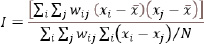 |
(1) |
The cluster and outlier analysis enables the identification of the locations of clusters on the map expressed in Equations (2) and (3).
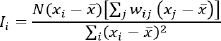 |
(2) |
 |
(3) |
where the value of Ii represents the localised Moran of province i.
Specifically, four types of spatial relationships can be obtained from LISA, namely, high-high (HH), low-low (LL), low-high (LH) and high-low (HL) [11-16]. The HH and LL categories designate positive spatial correlations, while the LH and HL categories indicate negative spatial relationships.
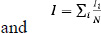
Furthermore, spatial regression analysis was conducted, utilising three models for examining spatial relationships: (1) ordinary least square (OLS), (2) SLM and (3) SEM. The OLS method is a simple model that considers relationships without taking spatial relationships into account. Spatial relationships are investigated using SLM, in which the dependent variable (suicide rate) of surrounding provinces influences the dependent variable (suicide rate) in the area being estimated (the province of interest), as shown in the following equation:
 |
(4) |
The value of Yi represents the dependent variable in the province of interest, while Yj stands for the dependent variable in neighbouring provinces located around the province of interest. The coefficient ρ denotes the degree of spatial dependence, Wij is the spatial weight matrix, Xi refers to the vectors of independent variables in the province of interest, β stands for coefficients of independent variables, and εi signifies the error term.
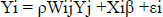
The spatial relationship can be alternatively examined by using SEM. Technically speaking, SEM allows the error term of adjacent provinces to influence that of the province under study, as represented in the following equation.
 |
(5) |
The value of Yi represents the dependent variable in the province of interest, while Xi denotes the independent variable in the province of interest. β represents the coefficients of independent variables, and μi is the error term. λ is the spatial error parameter, which reflects the degree of spatial influence caused by error terms of surrounding provinces (μj). Wij represents the spatial weight matrix that determines the criteria of spatial adjacency. εi signifies the disturbance in the province of interest.
When a significant spatial dependence was identified, SEM was performed but not OLS. The (robust) Lagrange multiplier (LM) test statistic [11] was used for determining which of the two models (i.e., SLM or SEM) would be suitable [12]. In situations where both models had statistically significant LM values, the model with the lower value was selected. The Akaike information criteria on (AIC) was used to find the model with the best fit, i.e., the lowest AIC value [13]
3. RESULTS
3.1. Univariate LISA
The univariate LISA results revealed statistically significant positive spatial dispersion, with LISA values ranging from 0.341 to 0.663 and p < 0.05 (as shown in (Figs. 1 and Table 1). In the cluster map of suicide rates for 2012, the provinces of Mae Hong Son, Chiang Mai, Lamphun, Lampang, Phayao, Phrae and Sukhothai formed a cluster of provinces with high rates of suicide and surrounded by a group of provinces with high levels of suicide. This finding was reflected in the results of the cluster map analysis, represented as an HH outcome. With changes over the past decade taken into consideration, the provinces of Mae Hong Son, Lampang, Phayao and Phrae still characteristically presented as an HH group in 2021 in Table 1 and Fig. (1).
| Variable | 2012 | 2013 | 2014 | 2015 | 2016 | 2017 | 2018 | 2019 | 2020 | 2021 |
|---|---|---|---|---|---|---|---|---|---|---|
| Suicide | 0.586 | 0.663 | 0.586 | 0.452 | 0.647 | 0.592 | 0.446 | 0.501 | 0.460 | 0.341 |
| NTL | 0.521 | 0.524 | 0.512 | 0.516 | 0.510 | 0.499 | 0.496 | 0.506 | 0.531 | 0.538 |
| Drug addiction | 0.259 | 0.229 | 0.166 | 0.213 | 0.060 | 0.205 | 0.167 | 0.232 | 0.181 | 0.380 |
| Divorce | 0.508 | 0.500 | 0.505 | 0.503 | 0.498 | 0.485 | 0.449 | 0.505 | 0.518 | 0.478 |
| Elderly | 0.393 | 0.425 | 0.444 | 0.428 | 0.442 | 0.462 | 0.475 | 0.487 | 0.501 | 0.507 |
| disabled | 0.526 | 0.544 | 0.561 | 0.548 | 0.596 | 0.592 | 0.156 | 0.534 | 0.536 | 0.570 |
| Poverty | 0.320 | 0.368 | 0.395 | 0.228 | 0.286 | 0.256 | 0.141 | 0.209 | 0.319 | 0.169 |
| Rainfall | 0.777 | 0.750 | 0.763 | 0.779 | 0.716 | 0.831 | 0.779 | 0.746 | 0.858 | 0.466 |
| NDWI | 0.827 | 0.851 | 0.836 | 0.852 | 0.833 | 0.830 | 0.833 | 0.833 | 0.837 | 0.830 |
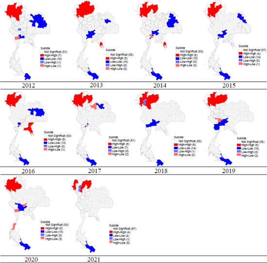
The Univariate Moran’s I of independent variables formed a cluster of provinces with high levels and were surrounded by a group of provinces with high levels of all independent variables. This finding was reflected in the results that showed positive spatial autocorrelation from 2012 to 2021 (Table 1).
3.2. Bivariate LISA
This section presents the results obtained by using bivariate LISA in relation to socioeconomic and physical geographical factors with suicide rates (Table 2, Figs. (2-9). This analysis is segmented into cases of suicide rates and eight variables, with the result of each bivariate analysis given below.
The bivariate Moran's I indicated significant statistical association patterns between independent variables and suicide rate (p-value < 0.05) from 2012 to 2021. There was a spatial correlation between the distribution pattern of the divorce rate, elderly population proportion, and disabled population proportion in the same direction as the suicide pattern. The outcomes of the bivariate LISA revealed a statistically significant positive correlation between the divorce rate, elderly population proportion, disabled population proportion, and suicide rate. In addition, the bivariate LISA revealed a statistically significant negative correlation between NTL density and average rainfall and displayed a negative correlation with suicide rates (Table 2).
| Variable | 2012 | 2013 | 2014 | 2015 | 2016 | 2017 | 2018 | 2019 | 2020 | 2021 |
|---|---|---|---|---|---|---|---|---|---|---|
| NTL | −0.157 | −0.339 | −0.212 | −0.212 | −0.173 | −0.160 | −0.309 | −0.216 | −0.287 | −0.122 |
| Drug addiction | 0.040 | 0.025 | 0.068 | 0.077 | −0.159 | 0.034 | −0.120 | −0.087 | 0.105 | 0.184 |
| Divorce | 0.340 | 0.279 | 0.325 | 0.295 | 0.356 | 0.378 | 0.173 | 0.196 | 0.204 | 0.375 |
| Elderly | 0.228 | 0.165 | 0.213 | 0.211 | 0.239 | 0.309 | 0.295 | 0.227 | 0.217 | 0.353 |
| disabled | 0.204 | 0.278 | 0.200 | 0.197 | 0.218 | 0.228 | 0.225 | 0.292 | 0.300 | 0.232 |
| Poverty | −0.021 | 0.117 | −0.031 | 0.016 | −0.064 | −0.030 | 0.100 | 0.013 | −0.179 | −0.126 |
| Rainfall | −0.097 | −0.123 | −0.138 | −0.158 | −0.216 | −0.362 | −0.305 | −0.077 | −0.210 | −0.021 |
| NDWI | 0.134 | 0.086 | 0.153 | 0.008 | 0.001 | −0.085 | −0.109 | −0.132 | −0.165 | −0.185 |
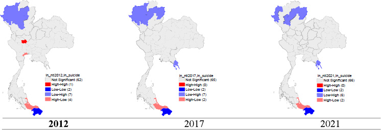
3.2.1. NTL and Suicide Rate
Fig. (2) shows an LH outcome for the provinces in the northern region, which are Mae Hong Son, Chiang Mai, Lamphun, Lampang, Phayao, Phrae and Sukhothai. Specifically, these provinces have low NTL but are surrounded by provinces with high suicide rates. With regard to changes over time within the past 10 years, the provinces of Mae Hong Son, Lamphun, Lampang and Phayao still maintained LH characteristics, and in 2021, the rates in Nan and Trat provinces increased (Fig. 2).
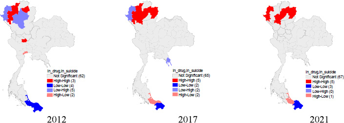
3.2.2. Drug Addiction and Suicide Rate
As delineated in Fig. (3), the provinces of Chiang Mai, Phayao, and Chainat emerged as concentrations of elevated drug addiction rates in conjunction with a proximal cluster of elevated suicide rates. This conclusion is drawn from the spatial cluster analysis that presents a high-high (HH) outcome. An examination of the temporal shifts over the past decade reveals that the provinces of Chiang Mai and Phayao sustained their HH characteristics, while the rates in Mae Hong Son, Lamphun, Lampang, and Nan provinces escalated in 2021. However, Chainat province did not exhibit any statistically significant variation (Fig. 3).
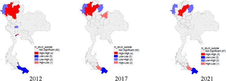
3.2.3. Divorce Rate and Suicide Rate
In the graphical representation provided by Fig. (4), the provinces of Chiang Mai, Lamphun, Lampang, Phayao, Phrae, and Sukhothai were discerned as regions with high divorce rates that corresponded with the high suicide rates in the surrounding regions in 2012. This is confirmed through the cluster map analysis, which demonstrates an HH outcome. When considering the evolution over the last decade, the provinces of Lamphun, Lampang, and Phayao perpetuated their HH patterns into 2021 (Fig. 4).
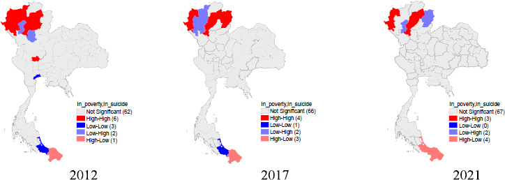
3.2.4. Poverty and suicide rate
According to Fig. (5), the provinces of Mae Hong Son, Chiang Mai, Lampang, Phayao, Phrae, and Chainat were identified as clusters exhibiting a high prevalence of poverty, coexisting with elevated suicide rates in their vicinity during 2012, leading to an HH outcome. Accounting for the shifts over the past decade, the provinces of Mae Hong Son, Lampang, and Phayao continued to exhibit HH characteristics in 2021 (Fig. 5).
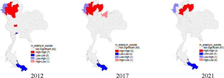
3.2.5. Proportion of elderly people and suicide rate
As evidenced by the spatial cluster map in Fig. (6), provinces such as Chiang Mai, Lampang, Phayao, Phrae, and Chainat were found to have a higher concentration of elderly residents, in tandem with elevated suicide rates in the surrounding areas. This scenario resulted in a high-high (HH) outcome. Reflecting on the changes over the preceding decade, the provinces of Lamphun, Lampang, and Phayao retained their HH characteristics. Interestingly,
Nan province demonstrated statistically significant values in 2021 (Fig. 6).
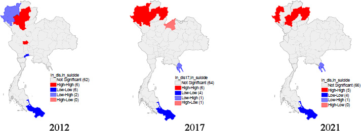
3.2.6. Proportion of Disabled Persons and Suicide Rate
Fig. (7) represents a spatial cluster map showcasing provinces like Lamphun, Lampang, Phayao, Phrae, Sukhothai, and Chainat, which in 2012 were characterized by a high proportion of individuals with disabilities, coupled with high suicide rates in adjacent regions. These factors culminated in an HH outcome. Considering the alterations over the previous decade, it was found that Lamphun, Lampang, and Phayao provinces persistently exhibited HH characteristics, with Mae Hong Son and Nan Provinces being incorporated in 2021. However, no statistical significance was discerned in the Chainat province (Fig. 7).
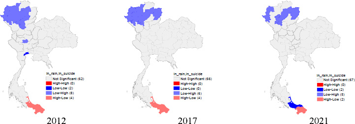
3.2.7. Rainfall and suicide rate
As shown in Fig. (8), in the 2012, spatial cluster map representing average rainfall, provinces including Mae Hong Son, Chiang Mai, Lamphun, Lampang, Phayao, Phrae, Sukhothai, and Chainat were identified as clusters with low average rainfall, yet they were bordered by provinces with high suicide rates. This dichotomy yielded a low-high (LH) outcome. Considering the alterations over the past decade, the provinces of Mae Hong Son, Lamphun, Lampang, and Phayao retained their LH characteristics, with Nan province demonstrating statistically significant levels in 2021 (Fig. 8).
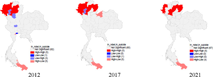
3.2.8. NDWI and suicide rate
The 2012 cluster map, as depicted in Fig. (9), showcasing NDWI disclosed that provinces, such as Mae Hong Son, Chiang Mai, Lampang, Phayao, and Phrae were characterised by a high waterlogged area and coincident high suicide rates. This confluence resulted in an HH outcome. Accounting for the transitions over the past decade, it was noted that Mae Hong Son, Lampang, and Phayao provinces upheld their HH characteristics until 2021, with Lamphun and Nan provinces newly included (Fig. 9).
3.3. Spatial Regression
The results were derived from the OLS regression analysis. The OLS models explained approximately 50.4%-74.3% of the suicide rate (R2 =0.504-0.743), respectively. The variables of average NTL density and average rainfall have an inverse relationship with the suicide rate (negative correlation). The divorce rate has a positive correlation and statistical significance (P < 0.001) for all the years under consideration. In terms of the proportion of the impoverished, the elderly, the disabled and NDWI have a positive correlation. However, the drug addiction rate did not show any statistically significant correlation (Table 3).
Table 4 demonstrates the results derived from the spatial lag model. The coefficient ρ, or the weighted average suicide rate of the surrounding provinces, affect the suicide rate of the province of interest (P < 0.05) for all years studied and explains approximately 56.3%-76.2% of the suicide rate (R2 =0.563-0.762). With regard to other independent variables, the NTL index and the divorce rate are statistically significant (P < 0.01) across all years. Other variables, such as the proportion of impoverished individuals, the elderly proportion, the average rainfall and NDWI, are statistically significant in certain years. However, the drug addiction rate and the proportion of disabled individuals did not show any statistically significant correlation (Table 4).
| Variable | 2012 | 2013 | 2014 | 2015 | 2016 | 2017 | 2018 | 2019 | 2020 | 2021 |
|---|---|---|---|---|---|---|---|---|---|---|
| NTL | -0.543 (0.106)*** |
-0.609 (0.090)*** |
-0.524 (0.105)*** | -0.480 (0.123)*** | -0.522 (0.125)*** |
-0.568 (0.121)*** |
-0.630 (0.132)*** |
-0.574 (0.129)*** | -0.773 (0.129)*** |
-0.421 (0.146)** |
| Drug addiction | 0.106 (0.074) |
0.088 (0.066) |
0.048 (0.061) |
-0.004 (0.137) |
-0.006 (0.064) |
-0.105 (0.094) |
-0.076 (0.133) |
-0.114 (0.106) |
-0.095 (0.091) |
0.059 (0.093) |
| Divorce | 1.384 (0.145)*** |
0.770 (0.113)*** |
0.830 (0.130)*** |
1.013 (0.164)*** |
1.106 (0.149)*** |
1.071 (0.152)*** |
0.833 (0.160)*** |
0.874 (0.150)*** |
0.773 (0.157)*** |
0.981 (0.156)*** |
| Poverty | 0.148 (0.055)** |
0.078 (0.068) |
0.023 (0.048) |
0.040 (0.066) |
0.055 (0.050) |
0.145 (0.080) |
0.084 (0.057) |
0.027 (0.055) |
-0.098 (0.080) |
0.197 (0.075)* |
| Elderly | 0.500 (0.333) |
0.888 (0.278)** |
0.357 (0.304) |
0.028 (0.320) |
0.413 (0.315) |
0.343 (0.283) |
0.152 (0.298) |
0.062 (0.301) |
-0.211 (0.325) |
0.268 (0.288) |
| disabled | -0.180 (0.226) |
-0.104 (0.186) |
0.138 (0.208) |
0.137 (0.157) |
0.042 (0.243) |
-0.151 (0.226) |
0.020 (0.066) |
0.450 (0.213)* |
0.142 (0.249) |
-0.184 (0.260) |
| Rainfall | -0.303 (0.238) |
-0.136 (0.181) |
-0.347 (0.174) |
-0.468 (0.207)* |
-0.238 (0.229) |
-0.501 (0.236)* |
-0.385 (0.204) |
-0.117 (0.168) |
-0.356 (0.195) |
-0.241 (0.211) |
| NDWI | 1.162 (0.290)*** |
0.414 (0.183) |
0.904 (0.227)** |
0.603 (0.207)** |
0.489 (0.243)* |
0.402 (0.264) |
0.153 (0.249) |
0.115 (0.170) |
0.233 (0.271) |
-0.209 (0.205) |
| Constant | 0.945 (0.813) |
0.350 (0.660) |
1.446 (0.625) |
1.704 (0.731)* |
1.046 (0.736) |
1.646 (0.809) |
1.650 (0.783)* |
1.035 (0.661) |
2.528 (0.721)*** |
1.147 (0.714) |
| F-stat | 24.238 | 22.867 | 17.437 | 13.322 | 14.261 | 16.085 | 9.766 | 12.663 | 10.85 | 8.513 |
| R2 | 0.743 | 0.731 | 0.675 | 0.614 | 0.630 | 0.657 | 0.538 | 0.601 | 0.564 | 0.504 |
| AIC | -68.984, | -97.945 | -83.97 | -60.760 | -63.302 | -79.646 | -54.901 | -77.089 | -63.88 | -75.204 |
| BIC | -48.008 | -76.969 | -62.993 | -39.784 | -42.326 | -58.669 | -33.924 | -56.113 | -42.910 | -54.228 |
| Log Likelihood | 43.492 | 57.973 | 50.985 | 39.380 | 40.651 | 48.823 | 36.450 | 47.544 | 40.946 | 46.602 |
| Variable | 2012 | 2013 | 2014 | 2015 | 2016 | 2017 | 2018 | 2019 | 2020 | 2021 |
|---|---|---|---|---|---|---|---|---|---|---|
| NTL | -0.470 (0.102) *** |
-0.493 (0.087)*** | -0.441 (0.101)*** | -0.399 (0.117)*** |
-0.409 (0.109)*** |
-0.442 (0.102)*** |
-0.432 (0.112)*** |
-0.443 (0.120)*** |
-0.627 (0.125)*** |
-0.358 (0.130)** |
| Drug addiction | 0.135 (0.068) |
0.122 (0.060) |
0.071 (0.056) |
0.023 (0.124) |
0.039 (0.054) |
-0.057 (0.076) |
-0.005 (0.114) |
-0.072 (0.090) |
-0.100 (0.080) |
0.056 (0.082) |
| Divorce | 1.193 (0.157) *** |
0.548 (0.118)*** |
0.685 (0.133)*** | 0.833 (0.163)*** |
0.813 (0.139)*** |
0.702 (0.138)*** |
0.560 (0.145)*** |
0.653 (0.134)*** |
0.589 (0.145)*** |
0.786 (0.147)*** |
| Poverty | 0.146 (0.050) ** |
0.061 (0.060) |
0.028 (0.044) |
0.031 (0.059) |
0.059 (0.042) |
0.071 (0.065) |
0.055 (0.049) |
0.032 (0.047) |
-0.077 (0.070) |
0.177 (0.066)** |
| Elderly | 0.485 (0.302) |
0.884 (0.246)*** | 0.386 (0.232) |
0.022 (0.288) |
0.407 (0.263) |
0.269 (0.229) |
0.068 (0.255) |
0.068 (0.255) |
-0.155 (0.286) |
0.162 (0.255) |
| disabled | -0.229 (0.205) |
-0.145 (0.165) |
0.069 (0.193) |
0.107 (0.141) |
-0.058 (0.204) |
-0.179 (0.182) |
0.067 (0.088) |
0.313 (0.181) |
0.056 (0.219) |
-0.239 (0.230) |
| Rainfall | -0.258 (0.218) |
-0.112 (0.161) |
-0.285 (0.161) |
-0.425 (0.194)* |
-0.180 (0.187) |
-0.319 (0.199) |
-0.304 (0.180) |
-0.150 (0.144) |
-0.345 (0.175) |
-0.283 (0.186) |
| NDWI | 0.966 (0.284) |
0.297 (0.168) |
0.724 (0.221)*** | 0.544 (0.193)** |
0.418 (0.207)* |
0.290 (0.237) |
0.188 (0.214) |
0.141 (0.145) |
0.256 (0.238) |
-0.135 (0.181) |
| Constant | 0.663 (0.757) |
0.047 (0.600) |
0.880 (0.610) |
1.560 (0.664) |
0.395 (0.635) |
1.077 (0.682) |
1.200 (0.699) |
0.811 (0.578) |
2.135 (0.666)** |
1.142 (0.632) |
| ρ | 0.212 (0.094) * |
0.283 (0.096)** |
0.213 (0.104)* |
0.241 (0.105)* |
0.391 (0.095)*** |
0.439 (0.092)*** |
0.403 (0.102)*** |
0.370 (0.097)*** |
0.310 (0.107)** |
0.318 (0.111)** |
| R2 | 0.761 | 0.762 | 0.696 | 0.644 | 0.707 | 0.748 | 0.614 | 0.676 | 0.618 | 0.563 |
| AIC | -71.479 | -103.243 | -85.903 | -63.674 | -75.435 | -96.266 | -62.669 | -87.5 | -69.635 | -80.482 |
| BIC | -48.171 | -79.935 | -62.596 | -40.367 | -52.128 | -72.958 | -39.362 | -64.192 | -46.328 | -57.174 |
| Log Likelihood | 45.739 | 61.621 | 52.951 | 41.837 | 47.717 | 58.133 | 41.335 | 53.75 | 44.817 | 50.241 |
| LMlag | 0.039 | 0.020 | 0.077 | 0.046 | 0.0002 | <0.001 | 0.015 | 0.0002 | 0.004 | 0.012 |
| Variable | 2012 | 2013 | 2014 | 2015 | 2016 | 2017 | 2018 | 2019 | 2020 | 2021 |
|---|---|---|---|---|---|---|---|---|---|---|
| NTL | -0.539 (0.104)*** |
-0.579 (0.088)*** | -0.507 (0.102)*** | -0.471 (0.121)*** | -0.506 (0.129)*** | -0.469 (0.123)*** | -0.576 (0.129)*** | -0.641 (0.134)*** |
-0.740 (0.131)*** |
-0.416 (0.145)** |
| Drug abuse | 0.114 (0.069) |
0.086 (0.061) |
0.056 (0.058) |
0.031 (0.125) |
0.016 (0.053) | -0.081 (0.085) |
-0.042 (0.127) |
-0.082 (0.101) |
-0.089 (0.084) |
0.076 (0.089) |
| Divorce | 1.354 (0.143) *** |
0.691 (0.113)*** |
0.801 (0.126)*** |
0.905 (0.164)*** | 0.911 (0.148)*** | 0.772 (0.151)*** | 0.689 (0.161)*** | 0.595 (0.160)*** |
0.636 (0.157)*** |
0.866 (0.156)*** |
| Poverty | 0.143 (0.048) ** |
0.065 (0.063) |
0.025 (0.045) |
0.030 (0.059) |
0.061 (0.042) |
0.054 (0.069) |
0.059 (0.052) |
0.004 (0.048) |
-0.098 (0.081) |
0.184 (0.067)** |
| Elderly | 0.389 (0.304) |
0.889 (0.262)*** | 0.376 (0.289) | 0.036 (0.296) |
0.457 (0.285) | 0.422 (0.257) |
0.108 (0.281) |
0.260 (0.278) |
-0.123 (0.313) |
0.238 (0.279) |
| disabled | -0.196 (0.205) |
-0.083 (0.172) |
0.129 (0.197) | 0.073 (0.140) |
-0.145 (0.229) | -0.267 (0.207) |
0.053 (0.095) |
0.127 (0.201) |
0.020 (0.240) |
-0.282 (0.243) |
| Rainfall | -0.372 (0.228) |
-0.185 (0.178) |
-0.353 (0.170)* | -0.639 (0.217)** | -0.315 (0.227) | -0.668 (0.253) |
-0.483 (0.214)* | -0.460 (0.195)* |
-0.455 (0.205)* |
-0.295 (0.203) |
| NDWI | 1.220 (0.294) *** |
0.429 (0.193) |
0.882 (0.226)*** | 0.694 (0.228)** | 0.586 (0.283)* | 0.675 (0.317)* |
0.232 (0.275) |
0.222 (0.212) |
0.242 (0.279) |
-0.155 (0.229) |
| Constant | 1.252 (0.751) |
0.475 (0.625) |
1.151 (0.630) |
2.188 (0.722)** |
1.145 (0.651) | 1.761 (0.772)** |
1.978 (0.780)* |
1.909 (0.645)** |
2.727 (0.700) |
1.391 (0.668)* |
| λ | 0.273 (0.128) * |
0.210 (0.133) |
0.148 (0.137) |
0.263 (0.129) | 0.479 (0.107)*** | 0.515 (0.103)*** | 0.219 (0.133) |
0.509 (0.104)*** |
0.246 (0.131) |
0.273 (0.128)* |
| R2 | 0.762 | 0.740 | 0.678 | 0.633 | 0.702 | 0.728 | 0.549 | 0.671 | 0.583 | 0.530 |
| AIC | -72.968 | -99.462 | -84.463 | -63.097 | -74.065 | -90.353 | -55.738 | -85.072 | -65.907 | -77.647 |
| BIC | -51.991 | -78.485 | -63.486 | -42.120 | -53.089 | -69.376 | -34.762 | -64.095 | -44.930 | -56.671 |
| Log Likelihood | 45.484 | 58.731 | 51.231 | 40.548 | 46.032 | 54.176 | 36.869 | 51.536 | 41.953 | 47.823 |
| LMerror | 0.038 | 0.411 | 0.635 | 0.285 | 0.005 | 0.020 | 0.778 | 0.030 | 0.266 | 0.324 |
Table 5 illustrates the results estimated via SEM. The coefficient λ, an indicator representing the spatial influences of the error term, holds statistical significance (P < 0.05) solely for the years 2012, 2016, 2017, 2019 and 2021 and explained approximately 76.2%, 70.2%, 72.8%, 67.1% and 53% of suicide rate (R2 =0.762, 0.702, 0.728, 0.671 and 0.530). With regard to other independent variables, the NTL index and divorce rates are statistically significant (P < 0.01) for all years. Other variables, including the proportion of impoverished individuals, the ratio of elderly people, the average rainfall volume and NDWI, exhibit statistical significance in certain years and correspond to theoretical expectations. However, variables such as the rate of drug addiction and the proportion of disabled individuals did not display any statistically significant correlation (Table 5).
4. DISCUSSION
In this present study, we aimed to identify a spatial association between socioeconomic factors, physical geographic factors and suicide in Thailand. Suicide rate clusters were found in the northern region of Thailand for the period from 2012 to 2021.
Our findings demonstrated the relationships between suicide rates and socioeconomic factors, physical geographic factors, such as divorce rates, poverty rates, elderly population proportions, and NDWI. These factors exhibited a positive correlation with suicide rates and were statistically significant. Conversely, the NTL density and average rainfall displayed a negative correlation with suicide rates, also with statistical significance.
One of the important findings of our study was the significant positive spatial correlation between divorce rates and suicide rates. With regard to divorce rates having a relatively persistent impact on suicide in the northern region of Thailand for the period from 2012 to 2021, previous studies indicated that divorce contributes to the onset of stress and anxiety due to problems arising from the accumulated stress of divorce-related issues, leading to suicidal ideation. In the initial stages of divorce, the risk of death by suicide increases by 1.6 times [14]. Divorce itself is an individual-level life event accompanying a high level of psychological distress, and on the aggregate level, which leads to family dissolution and social vary from culture to culture [5].
Our results indicated an association between the poverty rate and suicide rates. The poverty ratio represents the percentage of the population whose average monthly consumer expenditure per capita is below the poverty line, indicating the incidence of poverty [15]. A previous study found that poverty is associated with suicide rates in Japan [16]. Similarly, studies on the impact of socioeconomic conditions on the suicide tendencies of the Thai provincial population show that a higher poverty ratio results in an increase in suicide rates [2]. This result is consistent with studies on poverty and suicide among elderly South Koreans, which found that older individuals living in poverty have a higher risk of suicide compared with those with higher incomes [17].
Moreover, our study also revealed that the concentration of the elderly population correlated with the suicide rate. With regard to the elderly population ratio, the suicide rate among the elderly is higher than that of young adults due to loneliness in old age. Risk factors for suicide among the elderly include living alone, loss of a spouse, financial worries, deteriorating health and a high prevalence of mental health issues [18]. Similarly, research investigating suicide rates within the elderly population in China indicated that China ranks third globally in terms of the prevalence of suicide among the elderly. Remarkably, the suicide incidence within the rural elderly demographic is observed to be three to five times greater compared to their urban counterparts [19]. This finding is consistent with the results in the United States, where the elderly have the highest suicide rate of all age groups [20].
Our results indicated an association between the NDWI rate and suicide rates. NDWI can indicate the spatial and temporal variations of waterlogged areas [21]. Technically, this information is derived from remote sensing satellite imagery of water bodies [22]. Previous studies found frequent instances of drowning suicides in coastal areas or regions with harbours or large lakes [23]. This finding aligns with studies on the relationship between NDWI and suicide rates. The risk of living near a coastline has a positive correlation with increased suicide risk among the female population [24]. Similarly, access to water bodies contributes to an increase in suicides [25].
In our setting, NTL also predicts a significant negative correlation with suicide rates. The NTL density demonstrates urban boundaries that can be approximated from the density of night-time lights captured from satellites. This variable is another tool that can be used to analyse urban growth, reflecting areas with dense bright lights, which are indicative of economic growth [26]. Therefore, NTL density was useful in quantitatively characterizing the intensities of socioeconomic activities, urbanizations, and lifestyle [27]. As economic growth decreases, suicide rates tend to increase. In the case of China, the incidence of suicide among the elderly population residing in rural locales is notably three to five times greater compared to those seniors who inhabit urban areas [19]. This finding corresponds with a study on urban-rural disparities and suicide in Germany, which found that the rural population has higher suicide rates than the urban population [24]. This might be due to the rural area dweller having to face the risk factor affecting the living conditions because a health problem in a rural area is related to the transformation of environmental, social conditions, economic conditions, and culture.
Moreover, the average rainfall index also predicts a significant negative correlation with suicide rates. The average rainfall index can be used to explain the variation in agricultural yields and other economic variables, such as economic growth, poverty and inequality in agriculture and economics [28]. A study on the influence of socioeconomic and climatic conditions on the variations in suicide rates across the regions of Taiwan, using socioeconomic and climatic variables, found that climatic factors accounted for 59.0% of suicides [29]. In the case of Australia, a decrease in rainfall by approximately 300 mm increases suicide rates by about 8% [30].
CONCLUSION
Results from LISA and spatial regression methods reveal statistically significant spatial relationships between socioeconomic and geographical factors and suicide rates in Thailand. Higher suicide rates are primarily concentrated in provinces located in the northern region. Spatial regression analysis, utilizing the SLM and SEM methods, has shown a statistically significant relationship between various independent variables and the suicide rate. The distribution of divorce rates, poverty rates, elderly populations, and NDWI is particularly relevant, as these factors have exhibited a direct correlation with increased suicide rates.
According to the results of the current study, we recommend that socioeconomic and geographical factors should be considered in the planning and promotion of suicide measures in Thailand to improve the effectiveness of policies. The use of GIS is appropriate for different areas in Thailand, where there are differences in culture, traditions, and daily living [31, 32].
Therefore, the main findings of this study will be helpful for policymakers and medical practitioners to develop effective strategies concerning surveillance, control, and prevention for reducing suicide rates in a country. Specifically, the obtained analytical results would help the government in the northern region of Thailand, where the suicide rate is extremely high.
LIMITATIONS
Firstly, there are essential independent variables, such as alcohol consumption, household debt, the Gini coefficient, and incident rates of associated psychiatric disorders, which require inclusion in the analysis. Secondly, the secondary data were obtained from the Department of Mental Health, Ministry of Public Health and NSO of Thailand; therefore, there were limitations in terms of variables and data integrity. Future studies should investigate the reasons why this situation occurred; therefore, a qualitative study should be conducted to determine whether the cultural context and traditional lifestyle can confirm the findings of the quantitative method.
LIST OF ABBREVIATIONS
| NTL | = Night Time Light |
| SLM | = Spatial lag Model |
| SEM | = Spatial Error Model |
ETHICS APPROVAL AND CONSENT TO PARTICIPATE
Ethics approval was received from the Khon Kaen University Ethics Committee for Human Research (Reference No. HE662040).
HUMAN AND ANIMAL RIGHTS
No animals were used in this research. All human research procedures followed were per the ethical standards of the committee responsible for human experimentation (institutional and national) and with the Helsinki Declaration of 1975, as revised in 2013.
CONSENT FOR PUBLICATION
Informed consent was obtained from all participants.
STANDARDS OF REPORTING
STROBE guidelines were followed.
AVAILABILITY OF DATA AND MATERIALS
All data generated or analyzed during this study are available on request from the corresponding author [N.P].
FUNDING
None.
CONFLICT OF INTEREST
The authors declare no conflict of interest, financial or otherwise.
ACKNOWLEDGEMENTS
The authors would like to thank the Department of Mental Health for sharing health data.