All published articles of this journal are available on ScienceDirect.

Longitudinal Associations between Childhood Neighborhood Disadvantage and Young Adult Income
Abstract
Introduction:
This study examines the relationship between neighborhood disadvantage experienced in childhood and income level in young adulthood, with further assessment of whether that relationship is moderated by the duration of or age at exposure.
Methods:
Relationships between three types of neighborhood disadvantage (i.e., cohesion, quality, safety) at three developmental stages (i.e., childhood, early adolescence, adolescence) and income at age 25 (±1 year) were assessed among employed young adults using multivariable fixed effects models stratified by gender in a retrospective cohort of 660 U.S. youths drawn from a nationally representative panel study.
Results:
Findings demonstrated that childhood exposure to unsafe neighborhoods is negatively associated with income, but neighborhood cohesion and quality showed no effect. Further, the length of exposure to unsafe neighborhoods has a negative association with income among females (though not among males), but only for those residing in the most dangerous neighborhoods for the longest durations. Finally, the age of exposure provided statistically equivalent effects, indicating that there was no evidence that exposure timing mattered.
Conclusion:
These results suggest that a multi-faceted view of neighborhood disadvantage may be helpful in understanding its potential influence on adult economic achievement and raises questions about how these contexts are differentially experienced across genders.
1. INTRODUCTION
Since the 1980s, researchers have theorized that poverty is transmitted through the social and economic disadvantages of the neighborhoods in which people spend their lives, a construct known as “residential inequality” [1-4]. It is now widely accepted that the conditions and characteristics of the neighborhoods in which children grow up not only provide – or restrict – opportunities and quality of life but also are internalized into critical and potentially life-long patterns of beliefs and behaviors [5].
However, many studies of the impact of residential inequality on youth have focused on indirect measures, such as teen pregnancy or educational attainment, rather than direct measures of the relationships between childhood or adolescent neighborhood exposures on adult outcomes [6]. More recently, scientific inquiry on residential inequality has expanded to include the influence of the timing of neighborhood exposures in terms of the age at exposure and the cumulative duration of the exposure [6-8]. Several scholars have theorized that particular developmental phases may increase children’s vulnerability to internalize neighborhood effects [9-16], though debate continues whether stages in early childhood or adolescence are more susceptible.
The current study contributes to this discussion through an examination of the impact of neighborhood disadvantage during childhood on income in early adulthood, with additional analyses of whether that relationship is moderated by the duration of or age at exposure. Neighborhood disadvantage is typically defined as a lack of economic and social resources that are concentrated in certain neighborhood settings (e.g., limited access to nutritious food, violence, environmental exposures) [17-19], and disadvantaged neighborhoods are often characterized as experiencing “social dislocation” from mainstream culture (i.e., physically, economically, or socially isolated or displaced communities that experience increased social problems as a result) [6, 20].
The goals of this study were to assess the relationship between childhood neighborhood disadvantage and adult income and determine if that relationship was moderated by the length of time of the exposure or the age at which the exposure occurred. To this end, we analyzed nationally representative data from the Panel Study of Income Dynamics (PSID), the longest-running panel study in the U.S., to test the hypothesis that being exposed to greater levels of neighborhood disadvantage as a child would be associated with lower levels of income in adulthood among those employed. These data have not previously been utilized to assess the lasting effects of neighborhood cohesion, quality, and safety in childhood on adult economic outcomes, and, importantly, provide repeated measures across several developmental stages, thereby allowing analyses of the impact of the timing and duration of the exposures of interest.
2. MATERIALS AND METHODS
2.1. Study Population and Design
Study data were drawn from the PSID [21], which is a nationally representative longitudinal study of more than 22,000 households and the longest-running panel study in the U.S [22-24]. Initiated in 1968, PSID data are currently collected every other year [22] and include socioeconomic and demographic data on all household members, including several variables assessing annual income [24]. The children of PSID households are enrolled in the study when they are born or adopted [22, 23]. In 1997, the Child Development Study (CDS) was launched as a sub-study of children in PSID households to learn more about childhood and adolescence and contained several questions on neighborhood characteristics [25, 26]. The CDS collected information on 3,563 PSID children who were aged 0-12 years old in 1997 (CDS-I) [27]. These same children were surveyed again in 2002-3 (CDS-II; n=2,907) and in 2007-8 (CDS-III; n=1,506) [25]. When these children turned age 18 or 19 years (depending on the year data were collected), they were moved out of the CDS and into the PSID [24].
This study’s population was comprised of participants who: (1) were 5-9 years old at the time of CDS-I data collection, (2) were 10-14 years old at the time of CDS-II data collection, (3) were 15-18 years old at the time of CDS-III data collection, (4) had responses to all of the neighborhood exposure questions of interest in all three waves of the CDS, and (5) reported income >$0 (USD) at age 25 (±1) years in the PSID (2013, 2015, or 2017 waves). Thus, data were collected on each participant at four points in time: (Time 1) 1997 for participants when they were aged 5-9 years, (Time 2) 2002-3 for participants when they were aged 10-14 years, (Time 3) 2007-8 for participants when they were aged 15-19 years, and (Time 4) 2013-2017 for participants when they were aged 25 (± 1) years. Constructing the cohort in this way allowed each data collection timepoint to correspond to a generally accepted developmental age range, and the following designations from the American Academy of Pediatrics will be used: CDS-I = ages 5-9, or “childhood”; CDS-II = ages 10-14, or “early adolescence”; CDS-III = ages 15-19, or “adolescence”; and PSID = age 25 (±1 year), or “adulthood” [28, 29].
Of the 3,563 children who participated in the CDS-I, 1,589 (44.6%) were between the ages of 5 and 9 years old and had responses to the neighborhood questions. Of these, 1,435 (90.3%) were between the ages of 10-14 in 2002-3 and responded to the neighborhood questions; of these, 1,314 (91.6%) were between the ages of 15-19 in 2007-8 and responded to the neighborhood questions. When these 1,314 youths reached adulthood and were enrolled in the PSID, 660 (50.2%) reported >$0 income at age 25 (±1 year) and were included in this study; of those excluded, 89 (6.8%) reported their income as $0 at age 25 (±1 year), and 565 (43.0%) were non-responders. Thus, the total sample was 660 participants (males, n = 280; females, n = 380) who were followed, on average, for 18.5 years starting in 1997. At study start, the analytical sample was just over 55% female, with a mean age of 6.9 years and 74.5% identifying as White, 19.4% as Black, and 11.9% as Hispanic.
2.2. Measures
The independent variables were neighborhood cohesiveness, neighborhood quality, and neighborhood safety. These categories of neighborhood data were collected in each wave of the CDS from the child’s primary caregiver. Neighborhood cohesiveness was captured in the following questions: (1) “How difficult is it for you to tell a stranger in your neighborhood from someone who is a resident?” (Response options: very difficult, somewhat difficult, not at all difficult) and “How likely is it that a neighbor would do something if …” (2) “Your kids were getting into trouble?”, (3) “A child was showing disrespect to an adult?”, (4) “Someone was breaking into your home in plain sight?” and (5) “Someone was trying to sell drugs to your children in plain sight?” (Response options: very likely, likely, unlikely, very unlikely). Following other researchers, these responses were used to calculate a mean neighborhood cohesiveness score [6, 16, 30]. A single measure of neighborhood cohesiveness in each wave was constructed by taking the mean of the five component variables listed above. Cronbach’s alpha was calculated to check for internal consistency [31, 32], and all measures were acceptable [32] (0.7987 ≤ α ≤ 0.8432). Neighborhood quality was measured using the question: “How would you rate your neighborhood as a place to raise children?” (Response options: excellent, very good, good, fair, poor). Neighborhood safety was assessed using the question: “How safe is it to walk around alone in your neighborhood after dark?” (Response options: completely safe, fairly safe, somewhat dangerous, extremely dangerous).
The dependent variable was income at age 25 (±1 year). Once they reached adulthood, participants were asked several questions in each PSID wave about different sources of income in the previous year (e.g., wages, bonuses, overtime, tips, commissions, and additional job/practice/trade/miscellaneous labor income), which the PSID summed into a labor income variable. This study’s goal was to analyze labor income at age 25, but the PSID does not collect data every year. As a result, this study’s outcome variable was defined as participants’ income at age 25; if data were not collected at age 25, data provided at age 26 were used; if the data were missing at age 26, data provided at age 24 were used. Because the outcome of interest was income rather than employment status, individuals reporting $0 income during the year prior to data collection were excluded from the analytical cohort. A post-hoc sensitivity analysis was performed to determine if significant differences were evident between the members of the analytical sample and those excluded for reporting $0 income at age 25 or those lost to follow-up in adulthood.
Covariates that were considered for inclusion in the multivariable model included demographic, childhood, and adulthood variables. The demographic variables that were tested were gender, age, and race/ethnicity, which were available in all waves of the CDS and PSID. Childhood variables that were tested included individual measures of grade level, academic ability, self-perception, and social skills, as well as family measures of financial stability, family cohesion, and parenting approach and were available in at least one wave of the CDS. More specifically, the child-focused CDS variables assessed for model inclusion were current grade level, self-esteem, developmental delay diagnosis, academic giftedness, time management, feelings of discouragement about the future, global self-concept, and risk-taking behaviors (e.g., marijuana use, skipping school). Parent- and household-focused CDS variables assessed for model inclusion were household income, mother’s and father’s occupation, mother’s and father’s education level, number of household residents, number of siblings under age 18 residing in the home, whether the family was behind on bills or had money left at the end of the month, the number of household rules, the most important qualities children should have (e.g., be obedient, work hard), whether both parents were equally involved in childrearing, whether the benefits of parenting were worth the cost, degree of parenting strain, whether family members frequently criticize or hit, parental agreement about discipline, and parental warmth. Several interaction terms intended to represent the socioeconomic position of the parents were tested, including multiple combinations of occupation, education level, and income. Neighborhood-focused CDS variables considered for model inclusion were duration of neighborhood residence and observations of the neighborhood made by data collectors. The latter were used to construct a version of the Home Observation Measurement of the Environment, or HOME score. The current study’s HOME score was calculated as the mean of five descriptive neighborhood assessment variables (e.g., the presence of drug-related paraphernalia or garbage, the condition of the street and neighboring housing) in each wave in which it was available (CDS 2002-3 and 2007-8); then, a mean value for the HOME score was calculated across both waves, which is a standard approach [33]. Cronbach’s alpha was calculated for all HOME scores to assess internal consistency [31, 32], and all measures were acceptable [32] (0.7871 ≤ α ≤ 0.8418). Finally, adulthood PSID covariates that were tested for inclusion in the multivariable models included education level, occupation, and industry, which were collected in the same year as income.
2.3. Statistical Analyses
Initial univariate and bivariate analyses were executed to describe participants in terms of the independent and dependent variables and covariates, as well as to identify statistically significant unadjusted relationships. To determine the appropriate statistical approach for modeling the repeated exposure measures, results from an F-test and a Breusch-Pagan Lagrange Multiplier test were compared to assess evidence of fixed or random effects, respectively [34]; both types of effects were seen, and a subsequent Hausman test did not provide conclusive evidence on whether the data should be modeled as fixed or random [35]. Because the neighborhood of residence is not randomly selected, fixed effects models are frequently employed in studies of neighborhood impacts to reduce the potential bias arising from unmeasured individual characteristics contributing to neighborhood choice [6, 16, 36, 37]. Moreover, fixed effects models address issues of selection bias, omitted variable bias, endogenous membership, and time-varying responses beyond those related to neighborhood selection [16]. To model the relationship between the exposures and outcome of interest adjusted for sociodemographic, childhood, and adulthood variables, a step-down variable selection process was executed to identify a minimum sufficient adjustment set. Early in the multivariable modeling process, gender was identified as a confounder, and all analyses were stratified by gender. Other covariates that changed the measures of association by more than 10% were considered possible confounders and were re-tested in the model once it was reduced. Several interaction terms approximating childhood household socioeconomic position were tested, but none were significant, and no interaction terms are presented in the final models.
Because only those individuals reporting non-$0 income levels at age 25 (± 1 year) were included in the analytical cohort, the outcome of interest was zero truncated, with all outcome values positive. To determine whether the transformation of the dependent variable was necessary to satisfy the underlying assumptions of the regression model, a series of tests and plots were executed to assess distribution, residuals, and fit. The distribution of the exposure and outcome variables were plotted and visually reviewed. Although linear regression models assume a normal distribution of the residuals rather than the variables, transformations that generate normally distributed variables also often yield normally distributed residuals. Thus, the Ladder of Powers was utilized to identify which transformation(s), if any, yielded a normally distributed income variable [38, 39]; of the nine transformations generated, the identity, square root, and log transformations were statistically significant. New variables for the square root and log of income were created, and bivariate and multivariable modeling were repeated with all forms of the outcome. The identity, square root, and log models were compared in terms of model fit, with the identity model generating the largest R-square value. Next, each model was assessed to determine whether the variance of the residuals was constant using a White’s test for heteroskedasticity [40] and visual inspection of weighted standardized residual plots [41], with the identity and square root transformations performing equally well. Given these results and bearing in mind the difficulty of interpreting transformed variables, it was determined that a fixed effects model [42-44] with probability weighting, family clustering adjustment, and robust standard errors was appropriate [45, 46] for assessing the relationship between the non-transformed dependent variable and the independent variables. The general form of the fixed-effects model was:
 |
where Y was the outcome of interest; α was the intercept; FF was the set of fixed family variables; TVIF was the set of time-varying individual and family variables; N was the set of neighborhood variables; β1, β2, and γ were coefficients for the fixed family, time-varying individual and family, and neighborhood characteristics, respectively; μ was an error term; i denoted the individual; and j denoted the family [6, 16]. Because childhood neighborhood disadvantage may influence adult income either directly or indirectly (e.g., reduced educational quality), both the unadjusted and adjusted models are presented. Findings from the unadjusted regression models are presented to estimate the overall effects – direct and indirect – of neighborhood attributes on adult income. Findings from the multivariable regression models are presented to estimate the direct effects of the variables on the outcome [47].
Additionally, moderator tests were performed with two variables: (1) duration of neighborhood residence and (2) the HOME score. Both the duration of residence and the HOME score were associated with the exposures and the outcome in the bivariate analyses and were unlikely to be on the causal pathway [48, 49]. Neighborhood residence duration – available in all CDS waves – was tested as a moderator by creating an interaction term, estimating its association and significance with the outcome of interest using linear regression, and plotting the slope of the interaction [50]. An analogous process was used with the mean HOME score.
Finally, a series of post-analysis tests were executed to determine whether age at exposure altered the relationship between neighborhood disadvantage and adult income. For the continuous exposure variable (i.e., neighborhood cohesion score), the Games-Howell test was executed [51]; for the ordinal exposure variables (i.e., neighborhood quality for raising children, neighborhood safety walking after dark), Mauchley’s test of sphericity and Levene’s test of equality of error variances were executed [52, 53]. In addition, a sensitivity analysis was executed to determine whether there were significant differences between baseline characteristics of the analytical sample and those excluded for reporting $0 income or not responding at the study end.
All statistical analyses were conducted using Stata Statistical Software MP-Parallel Edition, v. 15.1, with statistical significance defined as α < 0.05.
3. RESULTS
At this study’s baseline (Table 1), on average, cohort members were in the 1st grade, had not been diagnosed with developmental delays (97.8%), and were not considered academically gifted (85.6%). Participants generally reported high global self-concept (mean: 5.6 of 7.0). In terms of their family situations, the mean household income of participants’ families was $55,260, with almost half of the families reporting falling behind in paying their bills at least once in the past 12 months and 21.9% reporting not having enough money in the past month to make ends meet. Most participants’ parents reported that the benefits of parenting were worth the costs (87.3%) and scored in the middle of the parental strain scale (mean: 2.2 of 5). More than half of the participants’ parents reported discussing their child’s interests with them every day (54.3%). Participants’ parents also indicated that their families were neither frequently critical of each other nor did they sometimes hit each other (85.4% and 78.8%, respectively); however, the majority of parents reported that they “sometimes” or “often” disagreed with their partner/spouse/ex-spouse/co-parent about disciplining the participant (62.9%). In terms of neighborhood residence, the majority of participants’ parents reported their families had lived in their neighborhoods for ≥ 5 years (60.9%). Participants’ parents rated their neighborhood’s level of cohesiveness at the mid-point of the cohesiveness scale (mean: 2.0 of 4), and more than half indicated that their neighborhood’s quality for raising children was “good”, “very good”, or “excellent” (72.7%) and their neighborhood’s level of safety for walking around after dark was “fairly safe” or “completely safe” (82.1%). At baseline, there were no statistically significant differences between male and female participants in terms of demographic or household variables, including the exposures of interest.
| - | Total Cohort | Males | Females |
|---|---|---|---|
| n = 660 | n = 280 (42.4%) | n = 380 (57.6%) | |
| % | % | % | |
| Age at Study Entry | - | - | - |
| Mean (SE) | 6.9 (0.07) | 6.9 (0.11) | 6.9 (0.09) |
| Race | - | - | - |
| White | 74.5 | 77.4 | 72.2 |
| African American | 19.4 | 15.8 | 22.1 |
| Other | 6.2 | 6.8 | 5.7 |
| Hispanic | - | - | - |
| Yes | 11.9 | 8.6 | 14.4 |
| Grade Level at Study Entry | - | - | - |
| Mean (SE) | 1.8 (0.07) | 1.8 (0.11) | 1.8 (0.10) |
| Developmental Delay Diagnosis | - | - | - |
| Yes | 2.2 | 3.1 | 1.5 |
| Gifted Program Participant/ Ddvanced Academic Work | - | - | - |
| Yes | 14.4 | 17.2 | 12.2 |
| Household Income, $ | - | - | - |
| Mean (SE) | 55260.61 (3361.77) | 54633.15 (4632.99) | 55751.23 (4507.75) |
| Household behind on Bills in Past 12 Months | - | - | - |
| Yes | 49.1 | 45.4 | 51.9 |
| Duration of Neighborhood Residency | - | - | - |
| Less than 1 year | 8.2 | 8.6 | 7.8 |
| At least 1 year but less than 3 years | 14.8 | 11.9 | 17.1 |
| At least 3 years but less than 5 years | 16.2 | 18.6 | 14.3 |
| 5 years or more | 60.9 | 60.9 | 60.8 |
| Neighborhood Cohesiveness Scale (Range: 1-4) | - | - | - |
| Mean (SE) | 2.0 (0.06) | 2.0 (0.08) | 2.0 (0.06) |
| Neighborhood Quality for Raising Children | - | - | - |
| Excellent | 7.0 | 6.9 | 7.1 |
| Very good | 38.4 | 40.5 | 36.9 |
| Good | 27.3 | 22.0 | 31.2 |
| Fair | 21.9 | 27.1 | 18.1 |
| Poor | 5.3 | 3.5 | 6.7 |
| Neighborhood Safety after Dark | - | - | - |
| Completely safe | 17.4 | 16.9 | 17.8 |
| Fairly safe | 64.7 | 65.9 | 63.9 |
| Somewhat dangerous | 12.1 | 11.9 | 12.2 |
| Extremely dangerous | 5.8 | 5.3 | 6.1 |
At study end (i.e., age 25 ±1 years), participants reported a mean income of $29,977.08 (range: $40 - $190,000), with significant differences seen by gender. The mean income reported by males was more than $8,000 greater than the income of females ($36,481 vs. $28,337, respectively; P = 0.002) (Table 2). Additionally, male and female participants differed significantly in terms of their education, industry, and occupation but not in terms of the age at which their income was reported. Females had more years of education than males, as almost 20% more females than males pursued education past a high school diploma (P = 0.007). More females than males worked in the service industry (P = 0.004) and in non-manual occupations (P < 0.001). Males were more evenly split between service and non-service industries (58.0% vs. 42.0%, respectively) and manual and non-manual occupations (55.4% vs. 44.6%, respectively) than were the females (service: 73.9%; non-service: 26.1%; manual: 25.0%; non-manual: 75.0%).
| - | Total Cohort | Males | Females |
|---|---|---|---|
| n = 660 | n = 280 (42.4%) | n = 380 (57.6%) | |
| % | % | % | |
| Age at Study End | - | - | - |
| Mean (SE) | 25.4 (0.04) | 25.4 (0.05) | 25.3 (0.05) |
| Education Level at Study Conclusion ** | - | - | - |
| Less than high school | 3.3 | 4.5 | 2.3 |
| High school diploma | 26.2 | 34.7 | 19.5 |
| Some college or trade school | 25.3 | 19.0 | 30.2 |
| College degree | 27.0 | 25.7 | 28.0 |
| Graduate study | 18.3 | 16.1 | 20.0 |
| Industry ** | - | - | - |
| Service | 66.9 | 58.0 | 73.9 |
| Non-service | 33.1 | 42.0 | 26.1 |
| Occupation *** | - | - | - |
| Non-manual | 61.6 | 44.6 | 75.0 |
| Manual | 38.4 | 55.4 | 25.0 |
| Income at age 25 (±1 year), $ ** | - | - | - |
| Mean (SE) | 31911.23 (1260.62) | 36481.33 (2214.71) | 28337.78 (1370.80) |
| - |
Males n = 280 (42.4%) |
Females n = 380 (57.6%) |
||
|---|---|---|---|---|
| Coefficient ($) | (95% C.I.) | Coefficient ($) | (95% C.I.) | |
| Neighborhood cohesiveness scale | -5222.51 | (-8802.76, -1642.26) | -2232.51 | (-4745.93, 280.90) |
| Neighborhood Quality for Raising Children | - | - | - | - |
| Excellent | Ref. | - | Ref. | - |
| Very good | -6632.50 | (-14813.16, 1548.17) | -947.59 | (-6959.39, 5064.21) |
| Good | -16190.20 *** | (-24570.64, -7809.77) | -6770.63 * | (-12808.50, -732.75) |
| Fair | -14712.12 ** | (-24518.16, -4906.09) | -8567.15 ** | (-14985.71, -2148.60) |
| Poor | -21252.57 *** | (-29800.35, -12704.80) | -5412.46 | (-16773.95, 5949.04) |
| Neighborhood Safety after Dark | - | - | - | - |
| Completely safe | Ref. | - | Ref. | - |
| Fairly safe | -6464.88 * | (-12747.98, -181.78) | -4036.72 | (-8286.71, 213.28) |
| Somewhat dangerous | -16281.06 *** | (-22858.68, -9703.45) | -7928.76 ** | (-12863.17, -2994.36) |
| Extremely dangerous | -21990.19 *** | (-29037.75, -14942.63) | -9709.29 * | (-18617.93, -800.64) |
3.1. The Impact of Childhood Neighborhood Safety on Adult Income
The stratified unadjusted analyses of exposure and outcome (Table 3) demonstrated significant differences between males and females, primarily in terms of the magnitude of the associations. Decreasing levels of neighborhood cohesiveness in childhood were associated with decreasing levels of income in males but not in females (P = 0.004 vs. P = 0.082, respectively). Decreasing levels of neighborhood quality for raising children and neighborhood safety after dark were associated with decreasing levels of income in adulthood among both males and females, but the magnitudes of association for the males were consistently more than twice that of females, on average. For example, being raised in an “extremely unsafe” neighborhood was associated with a decrease in income of $21,990 among adult males but only a decrease of $9,709 among adult females (P < 0.001 vs. P = 0.033, respectively).
| - |
Males n = 280 (42.4%) |
Females n = 380 (57.6%) |
||
|---|---|---|---|---|
| Coefficient ($) | (95% C.I.) | Coefficient ($) | (95% C.I.) | |
| Neighborhood cohesiveness scale | 222.39 | (-4671.95, 5116.72) | 1498.292 | (-1439.88, 4436.46) |
| Neighborhood Quality for Raising Children | - | - | - | - |
| Excellent | Ref. | - | Ref. | - |
| Very good | -3369.80 | (-13680.38, 6940.79) | -115.69 | (-6669.97, 6438.58) |
| Good | -8615.05 | (-20701.89, 3471.79) | -442.62 | (-6842.42, 5957.18) |
| Fair | -56.85 | (-13941.98, 13828.27) | -1076.35 | (-8030.93, 5878.22) |
| Poor | -4758.50 | (-19534.93, 10017.92) | -1893.01 | (-10065.85, 6279.82) |
| Neighborhood Safety after Dark | - | - | - | - |
| Completely safe | Ref. | - | Ref. | - |
| Fairly safe | -1269.48 | (-8618.78, 6079.82) | -4359.71 * | (-8482.84, -236.58) |
| Somewhat dangerous | -8862.98 * | (-17673.55, -52.40) | -1444.414 | (-6897.81, 4008.98) |
| Extremely dangerous | -18793.29 ** | (-29563.27, -8023.31) | -1586.711 | (-10076.70, 6903.28) |
| Most Important Quality the Parent believes a Child should have | - | - | - | - |
| To be obedient | Ref. | - | Ref. | - |
| To think for himself/ herself | 5549.13 | (-1706.85, 12805.10) | 9616.88 ** | (3108.08, 16125.68) |
| To work hard | 13159.65 * | (2289.52, 24029.78) | 8409.81 * | (1564.79, 15254.84) |
| To help others when they need it | 8734.13 * | (9.24, 17459.02) | 1680.48 | (-6594.05, 9955.01) |
| Childhood household income (per $5,000) | 117.25 | (-91.18, 325.69) | 569.82 *** | (262.81, 876.84) |
| Education Level at Study Conclusion | - | - | - | - |
| Less than high school | Ref. | - | Ref. | - |
| High school diploma | 8210.01 * | (270.72, 16149.30) | 13540.46 *** | (6441.13, 20639.80) |
| Some college or trade school | 8294.12 | (-264.24, 16852.48) | 15307.95 *** | (8228.29, 22387.60) |
| College degree | 26171.61 *** | (15406.41, 36936.81) | 22115.35 *** | (14126.84, 30103.87) |
| Graduate study | 8363.80 | (-3994.39, 20722.00) | 15688.23 *** | (8240.74, 23135.72) |
| Occupation | - | - | - | - |
| Non-manual | Ref. | - | Ref. | - |
| Manual | 988.9573 | (-5367.12, 7345.03) | -4793.31 * | (-7796.09, -1790.54) |
| Parental strain scale | -3085.289 | (-7487.04, 1316.46) | -5789.783 *** | (-7981.18, -3598.38) |
The stratified multivariable analyses (Table 4) demonstrated that only the exposure of neighborhood safety in childhood was significantly associated with income in adult hood among males and females after adjusting for covariates; neither childhood neighborhood cohesiveness nor neighborhood quality were associated with adult income. Compared to males living in a “completely safe” neighborhood as a child, those who grew up in a “somewhat dangerous” neighborhood saw a decrease in adult income, on average, of $8,862 (95% Confidence Interval [CI]: -$17673, -$52; P = 0.049); living in an “extremely dangerous” neighborhood as a child was associated with a decrease in adult income, on average, of $18,793 (95% CI: -$29563, -$8023; P = 0.001). Among females, those who grew up in a “fairly safe” neighborhood saw a decrease in adult income, on average, of $4,359 (95% CI: -$8482, -$236; P = 0.038), compared to females living in a “completely safe” neighborhood as a child, but no other exposure categories were statistically significant. All models were adjusted in terms of childhood household income, the parental strain scale, the most important quality the parent believed a child should have, education level at age 25, and occupation at age 25.
3.2. Evidence of Moderation due to Neighborhood Residency Duration on Neighborhood Disadvantage and Income among Females
In the moderation analyses, duration of residence was shown to be a statistically significant moderator of neighborhood safety among females, with those who grew up in “extremely dangerous” neighborhoods for “five years or more” reporting income that was $17,285 less, on average, than those who lived in “extremely safe” childhood neighborhoods (95% CI: -$29879, -$4691; P = 0.007); residence duration was not a moderator among males, and the HOME score did not show evidence of moderation among males or females.
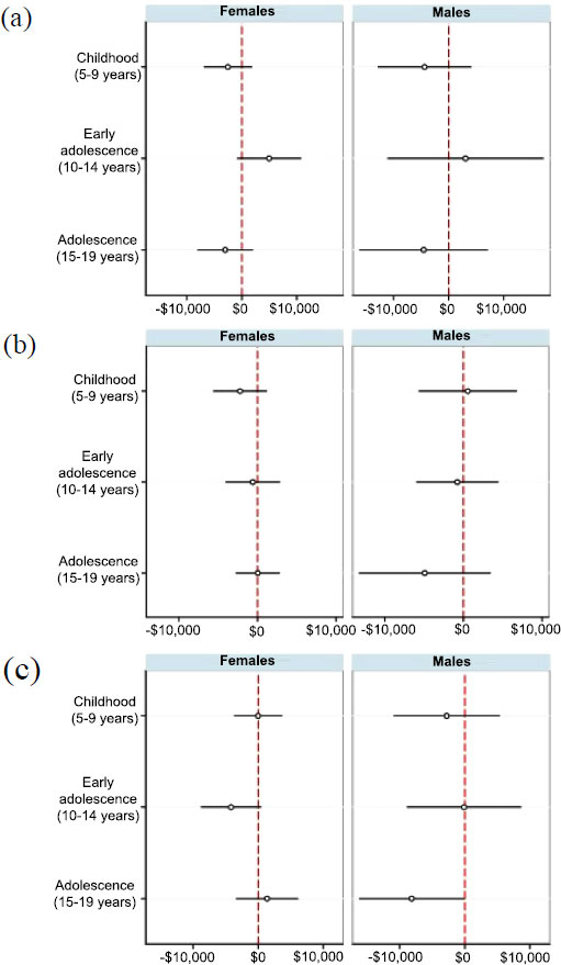
3.3. No Evidence of the Influence of Age of Exposure on Neighborhood Disadvantage and Income
In a series of post-hoc tests to determine whether the timing of exposure influenced the effect of neighborhood disadvantage on income, there was no evidence that the age of exposure significantly altered its relationship with the outcome, when compared to the same exposure at the other ages (Fig. 1).
3.4. Sensitivity Analysis Indicates Differences Between the Analytical Cohort and Excluded Adults
A sensitivity analysis was performed to determine whether significant differences existed between the baseline characteristics of the members of the analytical cohort compared to those adults excluded for reporting $0 income or due to non-response in adulthood. When compared to study participants at the study’s start, individuals who reported no income at age 25 (±1 year) were more likely to be Hispanic (P = 0.017), have been diagnosed with a developmental delay (P = 0.043), live in a financially unstable household (P = 0.037), or live in more dangerous neighborhoods (P = 0.028). Those who were lost to follow-up in adulthood were more likely to be male (P < 0.001), have been diagnosed with developmental delays (P = 0.025), or live in a household with lower levels of income (P = 0.004) than study participants at baseline. No differences were seen between participants and excluded individuals in terms of gender, race, academic giftedness, neighborhood cohesiveness, neighborhood quality, or residence duration.
4. DISCUSSION
This study examined the influence of neighborhood cohesion, quality, and safety in childhood on adult income and assessed whether the timing or duration of the exposures altered those relationships. Of the neighborhood characteristics
assessed, only neighborhood safety was associated with income in the adjusted models, with decreased safety linked to decreased income. Children and adolescents exposed to the stress of dangerous neighborhoods may become less engaged in school [54], withdraw from friends, or show symptoms of post-traumatic stress, such as irritability and intrusive thoughts [55], and they are at increased risk of reduced job stability in adulthood [56]. The psychosocial model of disadvantage argues that many disparities in health and well-being between socioeconomic groups arise because lower-resourced communities are more stressful living environments than well-resourced ones [3, 57]. If neighborhood conditions signify a dangerous environment, the community itself is perceived as an ever-present threat to residents, which has been associated with increased levels of allostatic load biomarkers [58-61] (i.e., indicators of the cumulative burden of chronic stress [62]). Residing in unsafe communities has been shown to impact the structure and function of children’s and adolescents’ brains in ways consistent with other forms of adversity, such as abuse or neglect [63-65], possibly due to the frequent flooding of the brain with stress hormones [66]. The resulting neurological changes have been linked to attention, learning, and cognitive limitations as well as declines in mental health and emotion regulation, any one of which may impact economic outcomes in adulthood [67, 68].
Marked gender differences were seen in terms of neighborhood safety relative to the level of perceived danger and the duration of exposure. Among males, decreasing levels of neighborhood safety were associated with decreasing earnings, which suggests a dose-response relationship, but there was no evidence that exposure duration modified this relationship. In contrast, exposure to unsafe neighborhoods among females was negatively associated with income only among those residing in the most dangerous neighborhoods for the longest durations (i.e., ≥ 5 years). The current results suggest that feelings of vulnerability related to decreasing levels of neighborhood safety are differentially internalized by male and female youths. Evidence demonstrates that ecological contexts of risk, including perceptions of danger and fear of crime [69], differ by gender, age, and income [70, 71]. Although perceived risk is generally higher among adult women than adult men [72], this pattern has been shown to be reversed in youths, especially among those residing in unsafe neighborhoods [73]. This may result from varying levels of neighborhood engagement across males and females, with females more likely to be shielded from risky situations by family and community members [74]. Greater protection of females (e.g., restricting with whom they socialize, setting earlier curfews) may account for the differential influence of family dynamics seen in these results, with parental preferences and stress levels related to adult outcomes among females but not males. Given the deleterious influence of long-term exposure to the most dangerous neighborhoods on females, however, this safeguarding may have limited effectiveness in the face of sustained adverse exposures. The concept of childhood exposure effects theorizes that accumulated neighborhood exposures in childhood effect adult outcomes, such as intergenerational mobility [75]. Several studies have demonstrated that such effects may differ by gender relative to neighborhood conditions [15, 75-79], with females showing greater benefits (e.g., increased college attendance, greater intergenerational mobility) when relocating to safer communities at younger ages [75, 76, 80].
Although greater neighborhood cohesion has been shown to reduce the impact of stressful events [81-83], this study did not demonstrate evidence of a relationship between neighborhood cohesion and income. Higher levels of neighborhood social cohesion support resiliency in children and adolescents [84, 85] and prevent mental health and behavioral problems [81]. Youths living in neighborhoods with lower levels of social cohesion are more likely to experience mental health distress, hyperactivity, or engage in indirect aggression [86]; conversely, increased levels of cohesion may increase child interaction with teachers and other adults in the community, contributing to school readiness among younger children and advances in social development amongst older children [86, 87], all of which may contribute to economic stability in adulthood. However, social cohesion has limited impact on complex situations [82], and the long-term economic outcomes of the current study may be beyond the influence of neighborhood cohesion.
In this project, neighborhood quality reflected parental perceptions of the objective and subjective characteristics of the community relative to raising children. In general, neighborhoods with fewer resources are perceived more negatively by residents, and individuals who indicate they chose their neighborhoods primarily for economic reasons score lowest on measures of neighborhood satisfaction [88]. Residing in less satisfactory neighborhoods is associated with lower-quality schools, limited access to safe outdoor spaces, and increased exposure to environmental hazards, all of which are associated with lower education attainment and reduced well-being among youths [89]. Among adolescents, perceived neighborhood quality is directly associated with self-esteem, self-efficacy, academic performance, and academic aspirations [90]. However, personal variables underlying neighborhood satisfaction strongly influence individual outcomes [91, 92], which may explain – at least in part – the absence of a relationship in this analysis between childhood neighborhood quality and adult income.
This study’s evidence of the association between detrimental neighborhood exposures and decreased economic outcomes is consistent with that of previous research [6, 11, 15, 16]. However, the preceding works did not present findings in terms of specific neighborhood characteristics (i.e., cohesion, quality, or safety) or stratified by gender; thus, we are not able to fully compare our more granular results with theirs. Several theories suggest that age of exposure alters the influence of neighborhood effects during particularly vulnerable stages, such as early childhood or adolescence [9-16]. Like Alvarado (2018), however, our results did not provide evidence that the timing of the exposure (e.g., the development stage in which the exposure occurred) influenced its relationship with the outcome. This may reflect differences in our study methodologies, particularly the definition of age cohorts and outcomes of interest.
This study’s findings should be viewed in terms of its limitations. Approximately 40% of adolescent CDS respondents were lost to follow-up in adulthood and, thus, excluded from this analysis. Statistically significant differences were seen between that population and the study cohort in characteristics that may influence economic outcomes in adulthood, including developmental delay diagnoses and lower levels of childhood household income, which suggests that non-response bias may be present in these results. Participants reporting no income in adulthood, whether due to intentionally (e.g., full-time students) or unintentionally (e.g., actively seeking employment) not working for wages, were also excluded from the study. This group differed from the analytical cohort at baseline in terms of greater ethnic diversity and increased likelihood of developmental delay diagnoses and of residing in financially unstable households and more dangerous neighborhoods. Additionally, exposure measures were reported by participants’ parents, which may have introduced bias into the data. Several of the neighborhood measures involved questions on sensitive topics, and some parents may have under-reported negative characteristics. Finally, only three waves of childhood data were available and only one wave of income was analyzed, which reduced the insights that could be gained from having additional waves of data for these analyses.
CONCLUSION
Despite these limitations, this study contributes key evidence on the long-term effects of neighborhood disadvantage in childhood. Although many topics related to neighborhood effects on children and adolescents are well studied, questions remain regarding long-term outcomes, in general, and economic outcomes in adulthood, more specifically. Further, findings have been mixed on whether exposure timing or duration mediates the influence of neighborhood attributes, with limited evidence on the mediation of long-term outcomes. This study addressed these questions and revealed that neighborhood safety in childhood may be a critical factor of economic outcomes in adulthood, exerting an influence not seen with neighborhood cohesion or quality. The differential impact of safety on males and females suggests that efforts to limit exposure to community-based intimidation, aggression, or violence should vary by gender as well as by severity and duration. Although our results highlight a lasting effect of reduced levels of neighborhood safety not demonstrated by neighborhood cohesion and quality, it is possible that the weakened social organization and control resulting from lower cohesion and quality may, in fact, contribute to lower levels of safety. Thus, these findings should be seen as underscoring the importance of comprehensive interventions targeting high-risk communities and vulnerable youth. Individuals cannot be separated from the structures and environments in which they live. If neighborhood disadvantage in childhood – and, specifically, neighborhood safety – influences income levels in adulthood, these individuals and their families may find themselves caught in a cycle of multi-generational disadvantage.
ETHICAL STATEMENT
In accordance with organizational research ethics procedures, this research was deemed exempt from review by a research ethics panel as this study was a secondary analysis of publicly available de-identified data and did not include contact with participants (i.e., U.S. 45 CFR 46.101(2)(b) Category 4) (https://www.hhs.gov/ohrp/regulations-and-policy/regulations/45-cfr-46/index.html).
CONSENT FOR PUBLICATION
Informed consent was obtained from a respondent household member at the time of Panel Study of Income Dynamics data collection.
STANDARDS OF REPORTING
STROBE guidelines were followed.
AVAILABILITY OF DATA AND MATERIALS
The Panel Study of Income Dynamics and PSID Child Development Supplement data analyzed in this study are publicly available from the University of Michigan Institute for Social Research Survey Research Center (https://psidonline .isr.umich.edu/).
The data analyzed in this study are publicly available from the Institute for Social Research Survey Research Center at the University of Michigan at [https://simba.isr.umich.edu /data/data.aspx], reference number [21].
FUNDING
None.
CONFLICT OF INTEREST
The authors declare no conflict of interest financial or otherwise.
ACKNOWLEDGEMENTS
Declared none.