All published articles of this journal are available on ScienceDirect.

Automatic Kidney Stone Detection System using Guided Bilateral Feature Detector for CT Images
Authors Info & Affiliations
Abstract
Background
Kidney stones, common urological diseases worldwide, are formed from hard urine minerals in the kidneys. Early detection is essential to prevent kidney damage and manage recurring stones. CT imaging has made significant progress in providing detailed information for disease diagnosis.
Aim
This study aimed to enhance kidney stone detection through advanced imaging and machine learning techniques.
Objective
The Guided Bilateral Feature Detector was proposed to identify and extract features for kidney stone detection in CT images. Unlike traditional filters like Gaussian and Bilateral filters, the Guided Bilateral Filter Detector prevented halo artifacts and preserved image edges by employing a guide weight. The extracted features were combined with the SVM algorithm to accurately detect kidney stones in CT images.
Methods
The proposed detector used the Guided Bilateral Filter to reduce the halo artifacts in the images and enhance the feature detection process. The detector operated in four stages to extract important features from CT images, and a 128-feature point generator provided a more detailed representation in aiding kidney stone detection and classification. The proposed detector combined with the Support Vector Machine algorithm to improve reliability and reduce computational requirements.
Results
Experimental results showed that the proposed Guided Bilateral Feature Detector with SVM outperformed existing models, including SIFT+SVM, SURF+SVM, PCA+KNN, EANet, Inception v3, VGG16, and Resnet50. The key performance metrics achieved included an accuracy of 98.56%, precision of 98.9%, recall of 99.2%, and an F1 score of 99%.
Conclusion
The findings indicate that the Guided Bilateral Feature Detector with SVM significantly enhances the accuracy and reliability of kidney stone detection, providing valuable implications for clinical practice and future research in medical imaging.
1. INTRODUCTION
The kidney is the most vital organ in the human body. Minerals in the urine cause solid particles, known as kidney stones. Kidney stones are common all over the world, with a frequency of about 12% around the world [1]. Kidney stones result from a synthesis of environmental and genetic influences. In addition, certain meals, drugs, being fat, and inadequate hydration can all contribute to it. Everyone, regardless of ethnicity, culture, or geo- graphy, is affected by kidney stones. This kidney stone is diagnosed by blood testing, urine tests, and scans. If the stone is not found right away, then surgery might be needed to remove it. One highly efficient method of correctly detecting the stone is by image processing. In the medical field, imaging is the most crucial element. Medical imaging techniques like CT, Doppler, and ultrasound are used by practitioners to evaluate the inside organs.
Currently, Machine Learning (ML) methods have been utilized to address the most challenging problems in urology health care [2]. Various imaging techniques like X-ray, Ultrasound, Computed tomography (CT), and so forth, with machine learning techniques, have been combined for diagnosing kidney stone disease [3, 4]. However, detecting kidney stone diseases using CT images has made significant progress by providing detailed information in the medical field for disease diagnosis.
2. LITERATURE SURVEY
The Plain Intensity filter were applied to US images to reduce and eliminate the addictive noise, and Symlets, Daubechies, and Biorthogonal wavelet sub-band filters extracted the features. The extracted features were subjected to segmentation using RD-LSS (Reaction-Diffusion - Level Set Segmentation). The ML models like Multilayer Perceptron, Back Propagation, Support Vector Machine (SVM), and Artificial Neural Network (ANN) were trained to identify kidney stones in US images with an accuracy rate of 98.9% [5]. Primary renal diseases like kidney stones, cysts, and tumors were detected with a total of 12,446 CT annotated images. Further, Six machine learning models, such as External Attention Transformer (EANet), Compact Convolutional Trans-former (CCT), Swin transformers, Resnet, VGG16, and Inception v3, were analyzed, and the results showed that the Swin transformer model outperformed the accuracy of 99.30% in diagnosing kidney tumors, cysts, and stones than other states of the art models [6].
A novel ExDark19 transfer learning-based classification was developed to identify kidney stones using CT images. The most informative feature vectors were selected using iterative neighborhood component analysis (INCA), and the chosen feature vectors were used for the K nearest neighbor (KNN) classifier along with the 10-fold cross-validation (CV) method. The model provided a 99.22% accuracy rate by 10-fold CV and a 99.71% accuracy rate by the hold-out validation method [7].
A two-stage segmentation method for CT images was proposed to diagnose kidney stones. Thefirst stage was employed to extract total kidney volumes, and the second segmentation stage extracted the stonepart. The five segmentation models, such as 3D UNet, Res U-Net, DeepLabV3+, SegNet, and UNETR 5, were provided for training the dataset, and a 5-fold CV classification algorithm was applied to classify the input CT images. The Res U-Net algorithm outperformed other algorithms and achieved the highest accuracy value of 99.95% [8].
A threshold-based segmentation for detecting stones in US kidney images was proposed, along with Merriman and Sethian methods, for smoothening curves and reducing shrinks in an input image. Morphological analysis was performed to determine the stone shape and location with a detection accuracy value of 96.82% [9]. The 3D U-Nets model was used for kidney stone segmentation with abdominal non-contrast CT images. The Deep 3D dual-path networks were implemented using hydronephrosis grading for automatic scoring of kidney stones. Thresholding and region growing were applied to detect and segment the stones using 3D U-Nets in the renal sinus region. The 5-fold cross-validation classification algorithm achieved an accuracy of 91.9% and a sensitivity of 95.9% using the test dataset [10]. The XRes-net-50 was proposed for kidney stone detection with 1799 CT images. The model used raw CT images as input and found the region of interest for accurate diagnosis. The model achieved an accuracy of 96.82% for CT images [11].
Kidney stone identification using SVM and KNN was proposed in US images. The US images were enhanced and filtered using Median and Gaussian Filter (GF), and images were sharpened by un-sharp masking. Morphological operations were used to find the final segmented image. PCA was used for feature reduction, and KNN and SVM classification algorithms were analyzed. Multilayer Perceptron (MLP) and PCA were used for feature extraction and reduction. Morphological operations were used to find the final segmented image. The segmented images were classified by KNN with an 89% accuracy rate and SVM with 84% accuracy rate [12].
Many researchers have used deep neural networks (DNNs) to detect kidney stones in images, and Table 1 provides the various techniques used for kidney stone detection. However, DNN-based methodology suffers from convolution operations, and it degrades the performance of the kidney stone detection system by using huge amounts of data with high computational costs. In this study, a conventional-based Guided Bilateral Feature Detector (GBFD) was proposed with less computational cost, which gave higher performance in detecting kidney stones.
| Author/Refs | Modality | Technique | Result |
|---|---|---|---|
| W. Preedanan et al., 2023 [3] | Abdominal x-ray images | Two-stage U- Net pipeline for segmenting urinary stones. | F2 Score =71.28% pixel-wise F2 score = 69.82% region-wise |
| W. Preedanan et al., 2022 [4] | Abdominal x-ray images | MultiResUnet model trained using GAN-based augmentation technique for segmenting urinary stone | F1 score = 69.59% pixel-wise F1 score = 68.14% region-wise |
| K. Viswanath et al., 2022 [5] | Ultrasound images | A preprocessing technique used a Plain Intensity filter. Symlets, Biorthogonal wavelet sub-band filters, and Daubechies have been used to obtain kidney stone features. Extracted features segmented using the RD-LSS (Reaction-Diffusion - Level Set Segmentation) method. | Accuracy = 98.9% |
| Islam, M.N et al., 2022 [6] | CT images | Six machine learning algorithms like EANet, CCT, Swin transformers, Resnet, VGG16, and Inception v3 | Swin Transformers Accuracy = 99.3%, Precision = 98.1%, Recall = 98.9%, F1Score = 98.5% and AUC= 99.97% |
| Mehmet Baygin et al.,2022 [7] | CT images | ExDark19 transfer learning-based classification model | 10-fold CV accuracy = 99.22% and Hold-out validation accuracy = 99.71% |
| Elton DC et al., 2022 [8] | CT images | Two segmentation stages, coarse segmentation and fine segmentation, are used for detecting stones. Five state-of-the-art segmentation algorithms have been considered for training. | Res U-Net = 99.95% |
| Angshuman Khan et al., 2022 [9] | Ultrasound images | Used PCA-based feature extraction method. | Accuracy = 96.82% |
| Cui, Y et al., 2021 [10] | Abdominal Non Contrast CT (NCCT) images | 3D U-Nets model used for kidney stone segmentation. Deep 3D dual-path networks were identified for hydronephrosis grading and the detection and segmentation of stones from the renal sinus region. | Sensitivity = 95.9% Classification AUC = 0.97 |
| Kadir Yildirim et al., 2021 [11] | CT images | XResNet-50 model | Accuracy = 96.82% |
| Nithya et al., 2020 [12] | Ultrasound images | ANN with k-means clustering algorithm | Accuracy = 99.61% |
| Verma et al., 2017 [13] | Ultrasound images | Median and Gaussian filters are used to enhance and sharpen an image. Morphological operations are used for segmented images. PCA is used for feature reduction. KNN and SVM classifications have been analyzed. | Accuracy of KNN = 89% Accuracy of SVM = 84% |
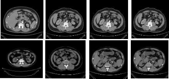
Sample images of normal and stone CT images.
3. MATERIALS AND METHODS
In this research, the cyst had 3,709 images, normal had 5,077 images, the stone had 1,377 images, and the tumor had 2,283 images, all combined in the dataset that had 12,446 CT images [14]. In this study, only the CT stone (1,377) and normal (5,077) images were considered and tested to prove the accuracy of the proposed GBFD+SVM model. The sample images of CT stone and Normal are shown in Fig. (1).
3.1. Guided Bilateral Feature Detectors
SIFT is the scale-invariant feature and was applied for pattern matching and recognizing an object in an image [15]. The robustness of the SIFT features was also applied in Magnetic Resonance Imaging (MRI) [16], remote sensing images [17], and so on.
The SIFT feature extractor smoothens the given images using a GF and it produces false edges when blurring the given image. The use of a Guided Bilateral Filter (GBF) in smoothening an image preserves the edges by using the guide weight along with the spatial and photometric weight of the Bilateral Filter (BF) but does not undergo gradient reversal artifacts [18]. The halo artifacts found in the GF produce false pattern matching on the images, which decreases the quality of the image. The halo artifact is a common problem in CT images, and it has to be addressed. Thus, reducing halo artifacts during the preprocessing step is important for finding good feature matching. Hence, a GBF was considered to reduce the halo artifacts and increase the performance of the feature detector.
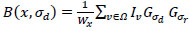
Fig. (2) illustrates the flow diagram of the proposed GBFD features and classification with the SVM model. The unenhanced input CT image was smoothed using GBF to reduce the noise and enhance that image for further processing. The smoothed CT image was given to the GBFD detector to extract features, and the descriptor was generated. These GBFD features were provided to the SVM for training and testing the dataset images.
The proposed GBFD feature detector consisted of four stages, the same as the SIFT method, to achieve better feature extraction and descriptor generation in order to classify the given images.
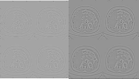
GF and BF [19, 20] are commonly used for smoothening an input image with an effort to increase the visual quality of the degraded image and also reduce the noise. A Guided Bilateral filter (GBF) preserves the edges similar to the BF and GF but does not undergo gradient reversal artifacts. In the GB filter, the guide weight is added along with the spatial weight and photometric weight of the BF. The guide weight gives more interesting information on the relationship between pixels than spatial weight. Fig. (3) shows the various filtered outputs for the normal and stone class CT images. The quality of the filtered image was measured with the common evaluating metric, such as the Peak Signal to Noise Ratio (PSNR) value. The PSNR value of the GF output was 35.95, the BF output was 36.67, and the GBF output was 37.89. The PSNR value was high, which means a good quality image, and GBF produced a higher PSNR value than GF and BF. Hence, GBF was considered for this study. Feature extraction was the next step to extract correct features for classifying the given image, and GBF Detector was proposed.
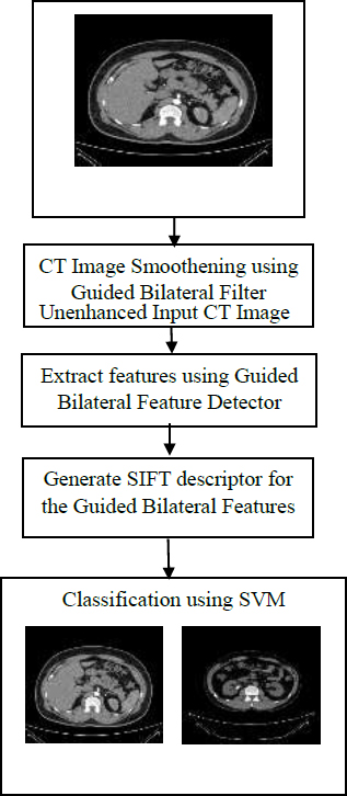
Flow diagram of proposed GBFD features with SVM model.
The proposed GBFD consisted of four stages, as in the SIFT feature detector, to achieve good feature extraction in CT images. Each stage of a GBFD is explained below.
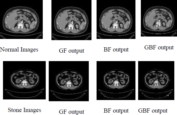
Filtered output images of normal and stone CT images.
3.1.1. Stage 1: Construction of Guided Bilateral Scale Space
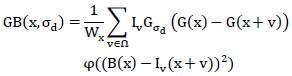
The construction of the GB scale space (Eq. 1) for an input image (Iv) of size M×N is defined as,
 |
(1) |
where the size of Ω is the part width of the GBF, x represents the pixel values of an image, B(x) denotes the BF output, v is the neighborhood of the center pixel, and wx is the normalization factor and is computed using Eq. (2).
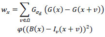 |
(2) |
where the scale space of a CT image as a function of B(x,σd) is,
 |
For various scales, B(x, kσd) and B(x, k2σd) are considered similar to the SIFT algorithm with scaling factor k, σd to Gaussian shape parameter in space, and Fig. (4) represents the different scaling of GB construction for an input image. In Eq. (3), Gσd and Gσr are the spatial weight and range weight, respectively,
 |
(3) |
where d(x,v) represents the Euclidean distance of x and v, δ(x,v) represents the intensity difference. G represents the guide image weight, and φ represents the photometric noise model.
Laplacian-of-Guided Bilateral (LoGB) has been computed using Eq. (4) by convolving the Laplacian filter L(x) with each Guided Bilateral image GB(x,σd)
 |
(4) |
Fig. (5) illustrates the output images of LoGB for each GB(x,σd). Maxima or minima of the LoGB pyramid is given an extrema point. Second-order Taylor series expansion provides a better extrema location to localize the feature point.
3.1.2. Stage 2: Feature Point Localization
Taylor series in the scale space LoGB(x,σd) eliminates the less contrast and badly localized interest points. The extrema point of less than 0.03 values was eliminated because it had an unstable extrema point. The edge-matching feature points were eliminated by using the Hessian matrix.

Guided Bilateral Scale Space construction of different scale value B(x, kσd) and B(x, k2σd) for input CT image.
Laplacian-of-Guided Bilateral (LoGB) for each Guided Bilateral Filtered input CT image.
3.1.3. Stage 3: Assignment of Magnitude and Orientation
The assignment of gradient magnitude m(x,y) and orientation Ɵ(x,y) for each Guided Bilateral smoothed image LoGB(x,σd) were computed using Eqs. (5 and 6), respectively. The orientation and magnitude were assigned for each feature point.
 |
(5) |
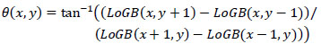 |
(6) |
The above equation computes the scale, orientation, and location for each feature point in CT images.
3.1.4. Stage 4: Descriptor Generation
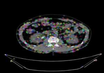
In the last step, the descriptors were generated by the computation of 16×16 neighborhoods of the pixel. At each feature point of the neighborhood, the gradient magnitudes and orientations were computed and weighted by Gaussian. The orientation histograms were created for each subregion of size 4×4 with 8 orientation bins. Finally, a vector had 4× 4× 8=128 elements. Fig. (6) shows the GBFD features for the input stone CT image.
GBFD features generated from the above stages were used for the SVM model to classify as normal or stone class.
3.2. Detection of Kidney Diseases using Proposed GBFD Features with SVM
SVM [21] is a classification mechanism with a minimum error rate and generalization. The GBFD features were used with SVM to classify the given images as kidney stone images or not. SVM separated the given data with a decision plane to decide the boundary between the two classes. SVM used training samples to construct the appropriate margin hyperplane and was largely used in non-linear regression and pattern classification challenges for better results. The normal and stone kidney CT images were trained using the kernel type of radial basis function of SVM.
GBFD features from stone CT input image.
3.2.1. Evaluation of Proposed GBFD
The evaluation of the kidney disease detection and classification was carried out on an Intel Core 5Y10C PC, 4 GB RAM, and Windows 10 for the CT images dataset, as presented in Fig. (2). Accuracy (Acc), Precision (Pre), Recall (Rec), and F1-Score (F1) were considered as the performance metrics by comparing the proposed GBFD features with state-of-art methods.
True positive (TP), False positive (FP), True negative (TN), and False negative (FN) samples were measured to find the Acc, Pre, Rec, and F1 values. The recall measured the model's ability to find sick patients with the disease in a given dataset of images. Recall defined the ratio of the number of TP and the number of TP plus the number of FN, which was calculated using Eq. (7).
 |
(7) |
Producing high Rec is trivial in the medical disease diagnosis field. Pre are predicted samples that are really positive. Pre defines the ratio of the number of TP and the number of TP plus the number of FP. High Pre is preferred in the medical disease diagnosis field and is calculated using Eq. (8).
 |
(8) |
Acc defines the ratio of the correctly classified samples to the total samples considered for evaluation, and the formula is defined using Eq. (9). The maximum value of accuracy is 1, and the least is 0.
 |
(9) |
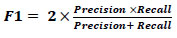
F1 value is a more comprehensive evaluation metric that unites precision and recall. F1 value is the formula defined by using Eq. (10).
 |
(10) |
4. RESULTS AND DISCUSSION
The most effective conventional feature detectors, such as SIFT, SURF, and PCA with SVM, were analyzed in this study, using the proposed GBFD+SVM for qualitative experimental analysis. In addition, four machine learning models, EANet, Inception v3, VGG16, and Resnet50, were considered for the performance comparison analysis.
The results of the SIFT+SVM, SURF+SVM, PCA+ KNN, EANet, Inception v3, VGG16, Resnet50, and Proposed GBFD+SVM were evaluated by calculating the performance metrics like Acc, Pre, Rec, and F1 values for the dataset images [14]. During the SVM training phase, 826 CT stone images and 3046 CT normal kidney images were considered in terms of a 60:40 ratio. For the SVM testing phase, 551 CT stone images and 2031 CT normal kidney images were considered. The extracted GBFD features were decided as an input to the SVM classifier.
In the SIFT+SVM training period, SIFT features with 112 dimensions were extracted from CT kidney images by 4X4 grids with 7 orientation bins. The extracted SIFT features were labeled and trained with SVM as normal or stone class. During the testing period, the test samples of SIFT features were applied to SVM in order to categorize the given sample as a stone or normal class.
Furthermore, 64-dimensional SURF features of a 4X4 grid with 4 orientation bins were constructed and given as input to the SVM classifier for the training and testing phase. Finally, SVM classified the given image as normal or stone class. SURF gave higher accuracy than SIFT by 0.6% and was also faster than SIFT.
| Methodology | Acc (%) | Pre | Rec | F1 |
|---|---|---|---|---|
| SIFT+SVM | 86.7 | 0.856 | 0.735 | 0.759 |
| SURF+SVM | 87.3 | 0.876 | 0.795 | 0.799 |
| PCA+KNN | 89 | 0.876 | 0.795 | 0.709 |
| EANet | 77.2 | 0.896 | 0.848 | 0.871 |
| Inception v3 | 61.60 | 0.584 | 0.898 | 0.708 |
| VGG16 | 98.20 | 0.985 | 0.973 | 0.979 |
| Resnet50 | 73.80 | 0.77 | 0.79 | 0.78 |
| Proposed GBFD+SVM | 98.56 | 0.989 | 0.992 | 0.990 |
Table 2 summarizes the performance of SIFT+SVM, SURF+SVM, PCA+KNN, EANet, Inception v3, VGG16, Resnet50 and Proposed GBFD+SVM considered in this study. From Table 2, the InceptionV3 model performed less with an Acc value of 61.60%. Resnet 50 and EANet provide moderate performance Acc values of 73.80% and 77.02%, respectively. VGG16 provides an Acc value of 98.20%, which is higher than SIFT+SVM and SURF+SVM Acc values of 86.7% and 87.3%, respectively. The proposed GBFD+SVM outperforms all the other models' accuracy by extracting the correct features to diagnose the presence or absence of kidney stones in the input images.
The Proposed GBFD+SVM provided reasonable Pre and Rec values of 0.989 and 0.992, respectively, by detecting kidney stone images. Higher Rec denoted the lowest possibility of miscategorizing the normal and stone class images. Figs. (7 and 8) show the systematic performance analysis of SIFT+SVM, SURF+SVM, PCA+KNN, EANet, Inception v3, VGG16, and Resnet50 with proposed GBFD+SVM for CT normal and stone dataset images. The comparative analysis shows that the proposed GBFD+SVM provides higher Pre, Rec, and F1 scores than SIFT+SVM, SURF+SVM, PCA+KNN, EANet, Inception v3, VGG16, and Resnet50 models by extracting stable features for detecting kidney disease in the given image.
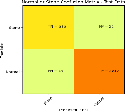
Fig. (8) shows the confusion matrix of the proposed GBFD+SVM for test dataset images. The actual normal images of 2031 and stone images of 551 were considered for testing the SVM with proposed GBFD features. The 2010 kidney normal images were appropriately predicted (TP), and 16 stone images were in normal class (FN). The model also misclassified 21 normal images (FP) and 535 stone images (TN) to the kidney stone class. Hence, evaluating these metric values is a necessary criterion for measuring the proposed GBFD+SVM performance.

Performance comparison of proposed GBFD+SVM for CT normal images.
Confusion Matrix of proposed GBFD+SVM for the test dataset.
Pre measures the rate of predicting kidney stones while recall gives the accurate prediction of positive values correctly, and the F1 score provides average harmonic values of Pre and Rec. The proposed GBFD+SVM model produced 98.56% Acc rate, 98.9% Pre rate, 99.2% Rec rate, and 99% F1 rate using 2582 test CT images.
CONCLUSION
This study focused on automatic kidney stone detection using GBFD features and presented SVM for classification. The use of a GB filter preserves the edges while smoothening an image and reducing the halo artifacts. The features extracted by GBFD showed robustness to noise compared to GF and BF. The proposed GBFD+SVM model performed considerably well in relation to Acc, Rec, Pre, and F1 values. The experimental result of the proposed GBFD+SVM was analyzed with six machine learning algorithms like SIFT+SVM, SURF+SVM, PCA+KNN, EANet, Inception v3, VGG16, and Resnet50 to prove the effectiveness for detecting and diagnosing kidney stone in CT images.
Furthermore, the confusion matrix obtained by the proposed GBFD+SVM was analyzed in terms of performance metrics of Acc, Rec, Pre, and F1 values to classify normal and stone classes. The systematic experiment results certainly showed that the proposed GBFD+SVM achieved a higher accuracy of 98.56%, which was comparably the same as the performance of other DNN models with less computation cost. In the future, to develop different disease detection systems, the proposed GBFD+SVM can be used for different imaging techniques.
AUTHORS’ CONTRIBUTIONS
It is hereby acknowledged that all authors have accepted responsibility for the manuscript's content and consented to its submission. They have meticulously reviewed all results and unanimously approved the final version of the manuscript.
LIST OF ABBREVIATIONS
| ML | = Machine Learning |
| CT | = Computed Tomography |
| RD-LSS | = Reaction-Diffusion - Level Set Segmentation |
| SVM | = Support Vector Machine |
| ANN | = Artificial Neural Network |
| EANet | = External Attention Transformer |
| CCT | = Compact Convolutional Trans-former |
| INCA | = Iterative Neighborhood Component Analysis |
| KNN | = K Nearest Neighbor |
| CV | = Cross-validation |
| DNNs | = Deep Neural Networks |
| GBFD | = Guided Bilateral Feature Detector |