All published articles of this journal are available on ScienceDirect.
AI-Assisted Breast Cancer Prediction, Classification, and Future Directions: A Narrative Review Involving Histopathological Image Datasets
Abstract
Breast cancer-related deaths in women have increased significantly in the past decade, emphasizing the need for an accurate and early diagnosis. AI-assisted diagnosis using deep learning and machine learning (DML) approaches has become a key method for analysing breast tissue and identifying tumour stages. DML algorithms are particularly effective for classifying breast cancer tissue images due to their ability to handle large datasets, work with unstructured data, generate automated features, and improve over time. However, the performance of these models is heavily on the datasets used for training, with the models performing inconsistently between different datasets. Given the prediction that by 2050, there will be more than 30 million new cancer cases and more than 10 million deaths worldwide, it is crucial to focus on recent advancements in DML algorithms and histopathological image datasets used in AI-assisted systems. Histopathological images provide critical information to identify tissue abnormalities, which directly impact model performance. This review discusses and analyses various DML-based models and the datasets used in their implementation, highlighting research gaps and offering suggestions for future improvements. The goal is to develop more effective and efficient approaches for the prediction of early-stage breast cancer. In addition, this early detection assists the healthcare professional in guiding prevention methods in smart healthcare systems.
1. INTRODUCTION
Breast cancer is the most common cancer in women, and its mortality rate has increased significantly in recent years. Breast cancer affects women primarily, and mortality rates in rural and economically depressed areas are higher than in developed ones. According to the International Agency for Research on Cancer (IARC), a branch of the World Health Organisation, approximately 2,261,419 new cases of breast cancer and 684,996 deaths occurred worldwide among people of all ages and genders. The number of cancer incident cases in India and various types of cancer incidence from 2020 to 2050 are shown in Fig. (1).
Breast cancer was considered to account for around 10% of cancers among diagnosed cancers in 2020, and 7% of death cases accounted for breast cancer [1]. Also, estimated that by 2050, there will be 38,25,471 new cancer cases and 10,37,723 deaths worldwide. Due to ignorance of the symptoms of the disease, early or late medical consultation leads to an approximately 33.8% increased mortality rate compared to the present rate. The shortage of healthcare professionals in rural areas contributes to a lack of timely and precise breast cancer detection, resulting in higher mortality rates. Using CAD technology, raising awareness about cancer symptoms, and implementing telemedicine-supported systems are solutions that aim to reduce mortality rates. Additionally, early detection and classification of breast cancer significantly decrease mortality rates.
The various imaging modalities [2], such as x-ray mammography, thermography, ultrasound, magnetic resonance imaging, and microscopic images, are available and used in the preparation of the data set. The histopathological image dataset plays a crucial role, and it influences model performance. Today, medical professionals can utilise these histopathological images in CAD systems to diagnose abnormal tissues. DML algorithms become an aid and beautify the CAD system in breast cancer diagnosis [3]. Generally, the deep CNN approach effectively extracted discriminate feature information from large datasets. In this regard, recent studies focused on the feature extraction and data evaluation of medical images to classify abnormal tissues. This investigation provides a survey of the most frequently used histopathological image dataset-based diagnosis with deep- and machine-learning CAD systems and its performance.
Biopsy screening is a technique for investigating breast tissue to inspect breast cancer. The pathologist took soft tissues from suspicious areas of a human body part and examined them on microscopic slides. The strained microscopic slides were transformed into digital colour images using whole-slide images (WSI). WSI colour images allow for the discrimination of various regions of interest (ROI) could be utilised in segmentation and feature extraction stages to train the model. The extracted features are selected and assigned to a particular class that is either invasive or non-invasive. A computer-aided detection process is that a computer yields to find out the location of suspected tissues. The development of CAD systems and advances in DML algorithms proved to overcome subjective errors. It improves the diagnosis rate and decreases the complexity of medical image analysis. Recent research revealed that the diagnosis sensitivity with CAD is better than that without CAD tools [4]. The studies exhibited that CAD tools combined with AI increase the precision of classifying the type of cancer. As a result, CAD has become the most dynamic study arena in medical image analysis to improve classification accuracy [5]. It helps to decrease false positive diagnosis reactions that may cause psychological stress, overdiagnosis, and treatment and is cost-effective. Furthermore, reduced false-negative diagnosis reactions, such as the omission of treatment, increase the mortality rate.
The major contributions of the paper are as follows:
- This comprehensive review investigates the research gaps in breast cancer diagnosis utilizing DML algorithms.
- The utilised dataset in the development model decides its performance.
- This review presents extensive literature related to breast cancer tissue classification based on different datasets and highlights the performance of these techniques.
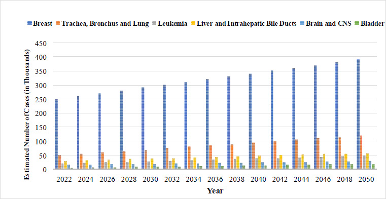
Projected number of cancer cases in India (2022-2050). [1] Source: Global Cancer Observatory.
2. Materials for Breast Cancer Classification
2.1. Basic Approach
The objective of this review is to compare various emerging approaches with respect to data sets utilised in the training of model for breast cancer categorisation. The primary objective of this review is to assess the response to the specified research inquiries during the development of a breast cancer detection system.
- How can the size and composition of a dataset impact the model's performance?
- What are the significant image preprocessing steps performed before being applied to the breast cancer categorisation system?
- Importance of the feature extraction method in the implementation of breast cancer categorisation systems?
- What are the performance metrics utilised to assess the developed breast cancer categorisation system?
Several research articles related to the breast cancer categorisation system and investigations were considered from 2010 to 2024. Emerging strategies used in the categorisation of breast cancer histopathological images as exposed in the following flow chart (Fig. 2).
All relevant studies on breast cancer were investigated; initially, a huge amount of research articles were composed due to the scope of the subject under study ‘classification of breast cancer “. Only some studies were included, while the rest studies were excluded because they were not developed with publicly available datasets and not tailored well with the predefined conditions of histopathological images. In this review, the studies included the previously mentioned datasets, machine learning approaches, and deep learning methods.
2.2. Datasets used
For the implementation of the breast cancer categorisation model, most of the researchers used bioinformatics and biomedical image datasets. From the associated work and literature study, it is concluded that the performance of the model depends on the type and size of the dataset used. Particular datasets utilised in specific model development produced good training and test accuracies, whereas the same model does not produce the same results with another database [6]. Thus, the data set plays a vital role in the implementation of model, performance, and comparison with specific models [7]. Thus, we discuss the most widely used datasets and DML-based models in the categorisation of breast cancer [8, 9].
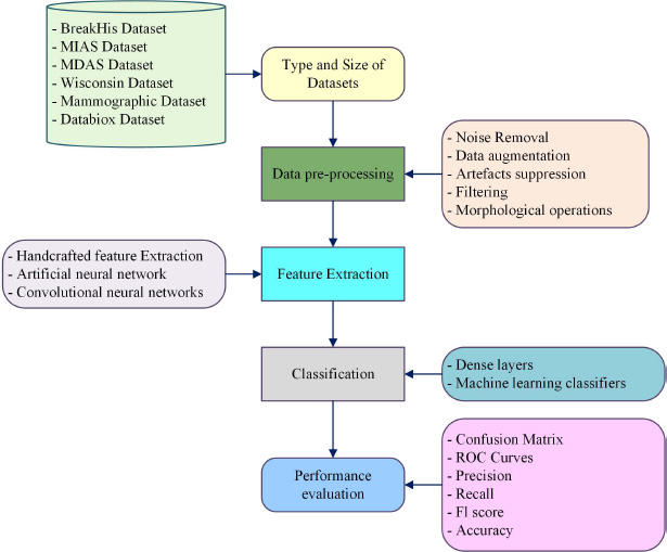
Flow chart of the breast cancer categorisation system
2.2.1. BreakHis Data Set
Most of the most advanced techniques use the BreakHis dataset, which is available online, free, and publicly [10]. Benign and malignant cancers are the most common types and there are four subclasses of each type. BreakHis data set contains histopathological images composed of 9109 breast tissues collected from 82 patients with various magnification factors 400x, 200x, 100x and 40x. It includes 2480 benign and 5429 malignant samples. Each image is a 3-channel RGB colour image with dimensions of 700x460 pixels, 8-bit depth in each channel and stored in PNG format.
2.2.2. Breast Cancer Wisconsin (Diagnostic) Data Set
It is another commonly utilised dataset in the breast cancer categorisation model, from the UCI repository; it is available for free and is an open-access dataset. Images were prepared from the specimen collected with a fine needle aspirate of breast tissues. The slides are digitised as histopathological images. The characteristics of these histopathological images are characterised by nuclei present in the image [11].
2.2.3. MIAS Database and DDSM Database
According to recent studies, the MIAS data set is widely used to develop breast cancer tissue classification models. This data set is readily available and accessible through the Mammographic Image Analysis Society (MIAS) database. The database follows the CSV file format [12].
2.2.3.1. DDSM Database
The Digital Database for Mammography Screening (DDSM) comprises 10,239 images, encompassing normal, benign, and malignant cases, all supported by verified pathology information. The DDSM dataset is also available online [13].
2.2.3.2. Databiox Database
The IDC-BC dataset, named Databiox, is a newly established database of histopathological microscopy images created by the Poursina Hakim Research Centre at Isfahan University of Medical Sciences in Iran. Compiled between 2014 and 2019, the dataset features specimens of breast tissues obtained from 124 patients. It includes a total of 922 images, classified into 259 for grade I, 366 for grade II, and 297 for grade III cancer, collected from 37, 43, and 44 patients, respectively. These images were captured at four different magnification levels (4x, 10x, 20x, and 40x) and are RGB colour images stored in JPEG format, with resolutions of 1276x956 and 2100x1574 pixels [14].
3. TECHNIQUES USED FOR THE CLASSIFICATION OF BREAST CANCER TISSUES
3.1. Approaches Used
The classification techniques used most frequently in the field of breast cancer categorisation as exposed in Fig. (3). First, we have a brief discussion of commonly used machine learning algorithms. After that, recent research and proposed studies were evaluated. Some classifiers provide a better accuracy level than other classifiers.
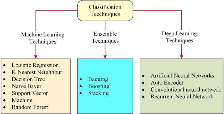
Popular classification techniques.
3.2. Machine Learning Techniques
Machine learning algorithms utilised for the categorisation of breast cancer tissue tasks are as follows:
- Logistic regression (LR): LR algorithm used for regression and categorisation problems to provide a continuous result and categorical outcome for a discrete task [15].
- K Nearest Neighbour (KNN): It was a supervised algorithm based on the calculation of the nearest neighbour. It is used for the recognition and classification of patterns. It works based on the distance between the target and its neighbours’ count categorised into a particular class [16].
- Decision Tree (DT): DT is an algorithm used for categorisation tasks and regression problems. A tree is formed on the threshold considered. The classification and regression tree (CART) is the subset of the decision tree approach [17].
- Naive Bayer (NB): This algorithm suits the large training dataset and produces fruitful results using the Bayesian approach. In a noisy environment, this approach could provide good accuracy [18].
- Support Vector Machine (SVM): The SVM is an algorithm used for categorisation and regression problems. In this, support vectors are formed, and based on these support vectors, the algorithm works. The SVM algorithm provides better accuracy with a large dataset [19, 20].
- Random Forest (RF):It is the most widely utilised supervised learning algorithm for addressing both categorisation and regression problems. Generally, the RF algorithm is utilised in the prediction of categorical class labels by fine-tuning a pretrained network [21].
3.3. Ensemble Techniques for Breast Cancer Categorisation
Ensemble is a technique utilised for homogeneous and heterogeneous algorithms to configure a new method for classification tasks.
- Bagging: The name implies that it bags the models. These models were trained separately and combined to perform the classification tasks [22].
- Boosting: A classification model formed by combining the weak models. Strengthen weak learners and boost their performance. The step-by-step implementation of weak models is trained individually and combined to increase their performance [23].
- Stacking: Combining weak models that were implemented based on different algorithms but using the same dataset. The name implies that heterogeneous algorithms merge to form a new model in the categorisation of breast cancer [24].
3.4. Deep Learning Techniques for Breast Cancer Categorisation
Deep network incorporated with multiple layer-based architectures used for the categorisation of breast cancer. Deep learning models are designed deeper to enhance the network’s ability to recognize and classify patterns into different categories.
- Artificial neural networks (ANN): With advances in computer technology, ANN is the most frequently used technique for data categorisation problems. Networks are incorporated with an input layer, hidden layers, and output layers. In ANN, each layer is fully connected with artificial neurons. These techniques are popular in the categorisation of patterns in the histopathological dataset. Algorithms are used to simplify complex problems with parallel processing, distributed memory, and collective solutions [25].
- Auto Encoder: The name implies that the input data and decoding is performed to get the original. The basic idea behind the encoder is to encode the important features from a huge number of datasets. The trained model ignores irrelevant and noisy information [26].
- Convolutional neural network (CNN): Convolution of image data with the kernels will extract features during the feature extraction phase. Various convolutional kernels were available for extracting features, reducing redundancy in features, and minimising complex calculations. Based on the type of filters, CNN layers are divided into convolutional layers, pooling layers and activation functions are generally successful in these layers. The final stage might be a fully connected layer or any conventional classifiers. It could classify the categorical dataset. All of these layers are combinedly and named CNN [27].
- Recurrent neural network (RNN): It is one form of a neural network that incorporated some hidden states. Hidden states utilise the output from the previous state as input for the next state and can undergo further processing through the concatenation of inputs using consistent parameters across each layer to simplify the architecture [28].
These techniques discussed in recent research work in the field of breast cancer categorisation and performance of the state-of-the-art research work evaluated in Table 1, considered the work done during the last decade. These work papers state that researchers developed different machine and deep-learning-based models to classify breast cancer. For training and testing of the developed model, different datasets were used.
3.5. Process for Model Performance Evaluation
The performance of the specific classification model is evaluated using widely used metrics. Commonly preferred metrics, such as precision, recall, F1 score, accuracy, receiver operating characteristics (ROC), and area under the curve (AUC), are typically used to assess the performance of the chosen model [29]. The following are the defined metrics, along with mathematical expressions. In this discussion, the class labelled as positive class and negative class used to refer to true positive or false positive based on model categorised into correctly or incorrectly labelled, respectively. The same can be extended to negative classes also.
| Authors | Year | Dataset Used | ML/DL Technique | Accuracy | Refs. |
|---|---|---|---|---|---|
| Mihir, et al. | 2007 | Wisconsin Breast Cancer database | SVM approach | 99.29% | [33] |
| Azar, Ahmad Taher, et al. | 2013 | Wisconsin Breast Cancer database | Multi-layer perceptron | 96.34, 97.66, 96.05% respective models | [34] |
| Abdel-Zaher, Ahmed M., | 2016 | Wisconsin Breast Cancer Dataset | Deep belief network path -Neural network (DBN-NN) | 99.68% | [30] |
| Teresa, et al. | 2017 | BreakHis dataset with magnification of 200× |
CNN+SVM | 83.3% | [41] |
| Mehrbakhsh, et al. | 2017 | Wisconsin Diagnostic Breast Cancer and Mammographic mass dataset | EM, CART, PCA and fuzzy rule-based techniques | 93.2% | [32] |
| Aditya, et al. | 2018 | Breast Cancer Histology Challenge (BACH) 2018 dataset | Transfer learning approach- Inception-V3 architecture | Patch-wise 79% Image-wise (2 class) 93% Image-wise (4 class) 85% |
[42] |
| Naresh, et al. | 2018 | MIAS Mammograph database. | Neural network | 98% | [36] |
| Yibao, et al. | 2018 | 30 H&E-stained histopathological whole slide images | Google Net | 98.46±0.40% | [39] |
| Meriem, et al. | 2018 | Wisconsin Diagnostic Breast Cancer | KNN and Naive Bayes classifier | KNN -97.51% NB -96.19% |
[31] |
| Zahangir et al. | 2019 | Two datasets-BreakHis and breast cancer classification challenge 2015 | Inception-v4, Residual Network and the Recurrent CNN combined | 97.57 ± 0.89% | [43] |
| Bibhuprasad, et al. | 2019 | Wisconsin Diagnostic Breast Cancer | PCA, ANN Multivariate statistical and ML techniques | PCA+ANN- 97% PCA+RF 95% |
[40] |
| Fung Fung, et al. | 2019 | MIAS dataset | CNN | 90.50% | [27] |
| SanaUllah et al. | 2019 | BreakHis and another dataset developed at the LRH hospital Peshawar, Pakistan. | Transfer learning approach | 97.525% | [35] |
| Ghulam, et al. | 2020 | BreakHis dataset | BMIC_Net model | 95.48% | [37] |
| Zheng et al | 2020 | The Cancer Imaging Archive (TCIA) Public Access | Deep-learning-assisted efficient AdaBoost algorithm |
97.2%, | [38] |
| Keping, et al. | 2021 | Breast pathology images from major hospitals via 5G | Transfer learning approach | 98.9% | [44] |
| Yu-Dong, et al. | 2021 | Breast mini-MIAS dataset | BDR-CNN-GCN algorithm | 96.10±1.60% | [45] |
| Dina A., et al. | 2021 | CBIS-DDSM and MIAS datasets | Multiple DCCNs, Fine-tuned CNN with SVM and PCA | --- | [46] |
| Abeer, et al. | 2021 | MIAS dataset | Transfer learning approach | 98.96% | [47] |
| Said, et al. | 2021 | BreakHis dataset | Transfer learning approach | Generalised | [48] |
| Hirra, Irum, et al. | 2021 | Four different datasets used | A novel patch-based deep learning method | 86% | [49] |
| Nusrat Ameen, et al. | 2021 | The IDC data set contains 162 H&E-stained whole slide images (WSI) | Ensemble of deep learning models | overall accuracy of 90.07% | [50] |
| Shallu, et al. | 2022 | BreakHis Dataset | Xception model and SVM classifier with kernel of radial basis function’ kernel | 96.25% | [52] |
| Shiksha, et al. | 2022 | BreakHis Dataset | Deep CNN with inception and residual blocks | 96.42% | [53] |
| Min, et al. | 2022 | BreakHis, IDC and UCSB datasets | Alex Net-BC model | 98.48% | [54] |
| Samriddha, et al. | 2023 | BreakHis Dataset | Gamma function-based Ensemble of CNNs | 99.16% | [55] |
| Saif Ur Rehman, et al | 2024 | BreakHis and the ICIAR2018-BachChallenge | GLNET model | 92.32% | [56] |
| Hasnae, a et al. | 2022 | BreakHis and FNAC dataset | Hybrid architectures using MLP | 99.00% | [57] |
| Hanan, et al | 2022 | BreakHis Dataset | Deep combination of ResNet 18, ShuffleNet, and Inception-V3Net | 99.7% | [58] |
| Saikat Islam, et al | 2022 | BreakHis and ICIAR datasets | Transfer Learning and feature extraction technique | 99% and 98% | [59] |
| Eelandula, et al. | 2023 | Databiox dataset | Ensemble of CNNs | 94% | [60] |
| Amel Ali, et al | 2023 | Digital Database for Screening Mammography (DDSM) dataset | Advanced Al-Biruni Earth Radius optimisation algorithm | 97.95% | [61] |
| Alaa Hussein, et al | 2024 | BreakHis Dataset | self-learning algorithm | 99.1% | [62] |
Precision: Precision is the ratio of true positives among the total positives redeemed or retrieved. Mathematically expressed as Eq. (1)
 |
(1) |
For a classification task, precision is about one of the particular class label predictions stated that the count of only true positives is divided by the total count of both true and false positive items categorised.
Recall: It is the ratio of true positives among the total retrieved and is mathematically expressed as Eq. (2)
 |
(2) |
For a classification task, recall is the count of true positives divided by the total count of items that belong to the positive class. Both precision and recall are based on true positives. However, precision and recall are inversely related; developing one at the cost of decreasing the other. For example, in the process of removing cancerous tissue, higher recall enhances the probability of eliminating healthy cells, as well as ensuring the removal of all cancerous cells. Increased precision reduces the likelihood of eliminating healthy cells while also minimising the risk of leaving behind any cancerous cells.
F1 score: In general, precision and recall metrics are inversely related. Precision and recall are together measured using new metrics called the F measure. The weighted harmonic means of precision and recall is called the F1 score. Mathematically expressed as Eq. (3)
 |
(3) |
Another metric utilised to gauge the classifier's performance is the true-negative rate, alongside accuracy. The true negative rate is also called specificity and is mathematically expressed as Eq. (4)
 |
(4) |
Accuracy: For only a balanced data set, precision metrics are used to evaluate the performance of the classifier. It can be a misleading measure for unbalanced data sets and mathematically expressed as Eq. (5)
 |
(5) |
Balanced Accuracy: To normalise the true-positive rate and true-negative rate, the mathematical average of the true-positive rate and true-negative rates is called balanced accuracy. Balanced accuracy can be used to measure the performance of the model trained with a balanced dataset or an imbalanced data set and mathematically expressed as Eq. (6)
 |
(6) |
ROC Curve: Adaptive identifiers for the receiver operating characteristic based on developers of these metrics. In 1941, military radar receiver operating characteristics were evaluated using these metrics. ROC is a plot, plotted between the true positive rate and the false-positive rate at various threshold points. It compared two operating characteristics, TPR and FPR, hence also called a relative ROC. The diagonal line in the plot divides ROC equally, and the points above the diagonal curve give good classification, whereas the below points represent bad results.
4. DISCUSSION AND FUTURE DIRECTIONS
The reviewed survey focuses on the research approaches used and results obtained for the classification of breast cancer using DML techniques [7]. The research literature on breast cancer classification using histopathological images and the research done so far are listed in Table 1. The study aims to review various DML algorithms that helped medical experts in the classification and prediction of breast cancer. The focus was on finding out the gap between the existing state-of-the-art techniques. This helps to improve the performance of the existing models. The existing research papers related to the DML algorithm on breast cancer classification and prediction were analysed. We categorised research papers into different sections and prepared a list based on their accuracy and the type of data set used.
4.1. Comparative Analysis of Various Classification Approaches
The highest accuracies achieved with a specific data set and DML algorithms are presented in (Table 2).
The various research works have been listed and the method that produces better performance with each datatype is listed in Table 2. Furthermore, the bar graph plot is plotted in Fig. (4).
4.2. Future Directions
This review analysis shows that the performance of the model is mainly influenced by the following factors. These are the research gaps to be filled by innovative and novel approaches compared with the state-of-the-art techniques in future work.
(i) The type of dataset employed for training and testing the model
(ii) The ML approach utilised for the provided dataset.
(iii) Type of CNN used to extract the features
(iv) Number of convolutional and pooling layers, number of epochs, type of activation function and optimisation techniques used in CNN.
(v) Transfer learning approach, where pre-trained model as the baseline model and fine-tuning with ML classifiers.
(vi) Ensemble approach – concatenation of networks.
However, for a particular dataset, the proposed model could work better instead of a specific other model and vice versa. As the dataset varied, the performance of a specific model also varied [63, 64]. Hence, we strongly noticed that the dataset is one of the significant aspects that impact the performance of the model. Therefore, hybrid, novel, and innovative approaches to combine the methods could be the future work.
| Dataset used | Approach | Accuracy | Refs. |
|---|---|---|---|
| Wisconsin Breast Cancer Dataset | Back-propagation neural network with Liebenberg Marquardt learning function from the deep belief network path (DBN-NN) | 99.68% | [30] |
| Breast Cancer Histology Challenge (BACH) 2018 dataset | Transfer learning large neural network architecture (Inception-v3) | 93% | [42] |
|
30 H&E-stained histopathological whole slide images (WSI). of ductal carcinoma in situ |
CNN model of Google Net performs well in histology image patch classification |
98.46±0.40% | [39] |
| Two datasets, including BreakHis and Breast Cancer classification challenge 2015 | Inception-v4, Residual Network, and Recurrent Convolutional Neural Network combined | 97.57 ± 0.89% | [43] |
| BreakHis and another dataset developed at the LRH hospital Peshawar, Pakistan. | Deep Learning Framework – Transfer learning | 97.525% | [35] |
| BreakHis Dataset | Deep combination of ResNet 18, Shuffle Net, and Inception-V3Net | 99.7% | [58] |
| The Cancer Imaging Archive (TCIA) Public Access | Deep-learning assisted efficient AdaBoost algorithm | 97.2% | [38] |
| Breast pathology images from major hospitals via 5G | The deep learning-based transfer learning approach | 98.9% | [44] |
| Mammographic image analysis- society (MIAS) dataset | Transfer learning approach | 98.96% | [47] |
| Databiox dataset | Ensemble of CNNs | 94.00% | [60] |
| Digital Database for Screening Mammography (DDSM) dataset | Advanced Al-Biruni Earth Radius optimisation algorithm | 97.95% | [61] |
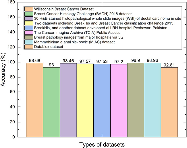
Comparative analysis of various types of datasets versus accuracy.
AI-assisted breast cancer prediction and classification can benefit greatly from fuzzy techniques and knowledge graphs, which offer methods for managing uncertainty, integrating intricate linkages, and enabling more comprehensive and interpretable systems [65, 66]. Improving explainability, integrating various data sources, increasing model accuracy, and guaranteeing widespread accessibility to AI-powered tools are key to the future of AI in breast cancer diagnosis. In addition to this, AI assisted real time diagnosis and decision support, AI for imaging modalities, and Integration with Health Records [67].
Large Language Models and Generative AI have the potential to significantly improve AI-assisted breast cancer classification and prediction. These technologies can help with decision-making, enhance model interpretability, enable individualised treatment plans, and create synthetic data for training.
Various viewpoints on the analysis of medical images, complementary methods for classifying and extracting features, understanding different deep learning architectures and their uses and techniques for enhancing the precision and dependability of detection, knowledge of various imaging modalities and their processing needs, increased the prediction and classification accuracy [68-72].
CONCLUSION
In this review article, various DML algorithms used for the categorisation of breast cancer are considered. Our main objective is to identify research gaps in breast cancer diagnosis and categorisation to reduce mortality rates. The most suitable algorithms that could extract the characteristics of histopathological tissue patterns were noticed. The main objective of this review study is to highlight up-to-date techniques and identify research gaps in DML algorithms that are used for the classification of breast cancer classification. In addition, list all existing review articles along with the research articles related to breast cancer and provide all the necessary and sufficient data to learners who want to work to gain knowledge about breast cancer categorisation using machine and deep learning techniques. The review of this study is performed through the kinds of datasets used for the implementation of models. To get some knowledge about recent trends, research gaps in the categorisation of breast cancer types, research articles, and the most used techniques deeply elaborated for the breast cancer categorisation. In the future, still, some research gaps still need to be filled by incorporating novel, innovative and hybrid algorithms with newly available datasets. This study discovered that alterations in the data set impacted the model’s performance. Researchers try to resolve the issue of limited dataset problems with the data augmentation approach even though there is a gap. Another issue is data imbalance, which could lead to bias towards a particular class. It needs to be resolved by proposing a new method.
AUTHORS CONTRIBUTION
G.N.: Contributed to the formal analysis, conceptualisation, data curation, methodology, validation, and visualisation and writing the original draft; R.P.Ch.: Validated, visualised and supervised the study; R.K.K.: Supervised the study; K.S.E.: Wrote – reviewed and edited the study.
LIST OF ABBREVIATIONS
| AI | = Artificial Intelligence |
| DML | = Deep Learning and Machine Learning |
| ML | = Machine Learning |
| DL | = Deep Learning |
| CAD | = Computer Aided Diagnosis |
| KNN | = Nearest Neighbour |
| SVM | = Support Vector Machines |
| ANN | = Artificial Neural Networks |
| RNN | = Recurrent Neural Network |
ACKNOWLEDGEMENTS
Declared none.

