All published articles of this journal are available on ScienceDirect.

Prevalence of Diabetes and Its Determinants among Kenyan Men in 2022
Abstract
Background
Diabetes affects millions of people worldwide and contributes to increased rates of sickness and mortality, making it a significant public health concern. Complete well-being depends on maintaining excellent health, and effective prevention and management of diabetes depend on understanding the factors associated with the disease. According to earlier research, the prevalence of diabetes varies by population, and men frequently have distinct risk factors from women. Therefore, identifying factors associated with diabetes in men is an essential problem that needs consideration.
Methods
The data employed in this study were obtained from the 2022 Kenya Demographic and Health Survey. Survey Logistic Regression models that consider the multi-stage features of the survey were implemented.
Results
The findings for this study are presented using a survey logistic regression model. The study findings revealed that the risk factors age, health status, hypertension, occupation, province, and wealth index were influential factors significantly associated with diabetes. The study also revealed that the interaction effects of age and health status, health status and wealth index, and health status and hypertension are strongly associated with diabetes.
Discussion
The findings highlight the complex interaction of socio-demographic, clinical, and economic factors in influencing diabetes risk among Kenyan men. Targeted interventions should prioritise older men, those in poor health, and those in lower wealth groups. The significant interaction effects emphasise the need for multifactorial prevention strategies. Public health policies should integrate routine screening, socioeconomic support, and workplace health programs to reduce the diabetes burden effectively.
Conclusion
The identified significant factors can inform the development of targeted strategies to reduce diabetes prevalence in Kenya. These findings emphasise the need for context-specific interventions focused on high-risk groups. Strengthening routine health screening and addressing social determinants are critical for effective diabetes prevention and control.
1. INTRODUCTION
Due to dietary choices, urbanisation, and changes in lifestyle, diabetes is becoming more and more common in today's culture, making it one of the most urgent public health issues. In the modern era, with globalisation, diabetes is a major reason for medical care expenditure and mortality, and it is one of the biggest health challenges of the current and future time frames [1]. Diabetes, scientifically referred to as diabetes mellitus, is a long-term condition that arises when the pancreas fails to generate sufficient insulin or when the body is unable to use it effectively. Insulin is a hormone that regulates blood glucose. Diabetes is a major cause of blindness, kidney failure, heart attacks, stroke, and lower limb amputation [2, 3]. It is one of the four priority non-communicable diseases (NCDs) that are targeted for action by world leaders [4]. The main types of diabetes are type 1 diabetes mellitus (T1DM), type 2 diabetes mellitus (T2DM), and gestational diabetes mellitus (GDM).
T1DM (insulin-dependent, juvenile, or childhood-onset diabetes) involves insufficient insulin production in the body and necessitates daily insulin administration [3]. Individuals with type 1 diabetes represent only 5% to 10% of the entire diabetic population. The precise cause of Type 1 diabetes remains unclear; however, it is believed to result from a mix of genetic and environmental factors, such as contact with a specific virus [5]. T2DM is characterised by hyperglycaemia caused by insufficient insulin production and the body’s inability to adequately respond to insulin [6]. T2DM is the most prevalent type of diabetes and is defined by insulin resistance. For decades, type 2 diabetes was regarded as an adult condition, but it has started appearing in children. T2DM represents more than 90% of all diabetes cases globally [7]. Ninety to ninety-five percent of all current diabetes cases are type 2 [3, 8].
Gestational diabetes is high blood sugar that occurs in certain women during pregnancy and typically resolves after giving birth. Both mother and child face a heightened risk of developing T2DM. Gestational diabetes occurs when your body is unable to produce sufficient insulin during pregnancy. Gestational diabetes can elevate the chances of hypertension during pregnancy and may lead to a larger-than-average infant, raising the possibility of a caesarean delivery [5].
Both the number of cases and the prevalence of diabetes have been steadily increasing over the past few decades, despite it being a preventable disease [9]. Without sufficient action to address the situation, it is predicted that 643 million people will have diabetes by 2030 [7, 10]. In comparison with the high-income countries, the prevalence of diabetes has increased more quickly in low- and middle-income countries during the past ten years. The age group with the highest diabetes prevalence in Africa is between 55 and 64 [6].
Since 2015, Kenya has acknowledged diabetes as a significant public health issue. In 2021, the total number of diabetes cases reached 821,500, reflecting a 3% prevalence rate among adults in Kenya [7]. A national survey indicated that the prevalence of type 2 diabetes was nearly twice as high in urban areas (3.4%) compared to rural regions (1.9%) [11]. Other studies have shown that the prevalence is even greater in low-income urban neighbourhoods within Nairobi, the capital of Kenya, ranging from 4.1% to 5.3% [11].
It was estimated that diabetes-related fatalities in Nairobi rose by 65% from 2009 to 2019, with diabetes listed among the top ten causes of death and disability in Kenya in 2019 [11]. In Kenya, non-communicable diseases (NCDs) represent 27% (284,000) of all deaths, with diabetes accounting for roughly 10,000 of those fatalities [12]. The expenses related to diabetes care, such as medications, blood glucose monitoring, and maintaining a healthy diet, can impose a considerable financial strain [13]. Managing diabetes in Kenya poses significant challenges, particularly for those from low-income families.
Many people are unaware of their diabetes status, especially in African communities, where there are insufficient resources related to health care. Reducing diabetes risk involves lifestyle changes such as a healthy diet, regular exercise, weight management, and avoiding smoking and excessive alcohol. Public health strategies like early screening, awareness campaigns, and policy regulations also play a vital role. Medical interventions, including blood sugar monitoring and medication for high-risk individuals, help in prevention. Stress management and regular health checkups further reduce the risk. Targeted interventions for high-risk populations can further improve outcomes. The purpose of this study is to identify the socio-demographic, health-related, and lifestyle factors associated with diabetes among men in Kenya by considering the multistage nature of the sampling design.
2. METHODS
2.1. Data Source
This study used secondary, deidentified data from the 2022 Kenya Demographic and Health Survey (DHS).
Kenya is one of the forty-eight nations in the IDF's African region. The Kenya Demographic and Health Surveys (KDHS) have been conducted in the years 1989, 1993, 1998, 2003, 2008-2009, 2014, and 2022. The 2022 Kenya Demographic and Health Survey (KDHS) was employed in this study. The Kenya National Bureau of Statistics (KNBS), in collaboration with the Ministry of Health (MoH) and other stakeholders, implemented the survey. The Kenya Household Master Sample Frame (K-HMSF) served as the source of the sample for the 2022 KDHS [14]. This sample frame is the frame that KNBS currently operates to conduct household-based sample surveys in Kenya. Kenya created 129,067 enumeration areas (EAs) due to its 2019 Population and Housing Census [14]. To generate the K-HMSF, 10,000 of these EAs were chosen with a probability proportional to their size. The 10,000 EAs were randomised into four equal subsamples, and the survey sample was drawn from one of these four subsamples. The EAs were developed into clusters through household listing and geo-referencing. Kenya has forty-seven counties, and each of the counties was stratified into rural and urban strata, resulting in ninety-two strata since Nairobi City and Mombasa counties are purely urban. The sample was a stratified sample selected in two stages from the K-HMSF. In the first stage, 1,692 clusters were selected from the K-HMSF using equal probability with independent selection in each sampling stratum [14]. Every chosen cluster had its households listed, and the list of households produced was used as a sampling frame for the second selection step, in which twenty-five households were chosen from each cluster [14]. Eight questionnaires were used for the 2022 KDHS to conduct the survey.
2.2. Study Variables
The response variable in this study is the presence of diabetes, which is a binary outcome (yes or no). The explanatory variables included in this study are age, region, ethnicity, place of residence, educational level, marital status, occupation, health status, wealth index, smoking status, alcohol consumption, and hypertension. Multiple researchers from past studies identified these variables as risk factors for diabetes [15, 16]. Some significant two-way interaction effects were also included.
2.3. Statistical Methods
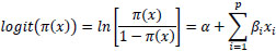
An outcome with two categories (e.g., consisting of ones and zeros) is called a binary outcome. Diabetes as the response variable is dichotomous because it consists of “yes” and “no,” which are used to identify whether an individual is diabetic or non-diabetic. A well-known mathematical modelling technique for simulating a dichotomous disease outcome is logistic regression [17, 18]. Diabetes lends itself to a logistic regression model, as it holds the properties of the model. Logistic regression is particularly valuable because the predictions from a fitted model are probabilities, constrained to be within the range of values 0-1 [19, 20]. Logistic regression is frequently utilised to model a binary variable (0 or 1) based on one or several predictor variables. This model assumes that the data is collected through a simple random sampling method. The logistic regression model can be mathematically defined as:
 |
(1) |
where π(x) = probability that a man will have diabetes, α is the intercept, βs are slope parameters, and Xs are explanatory variables for the model.
Nevertheless, a complex survey design was incorporated due to the DHS sampling technique. The data that is used in this study is survey data; there are certain elements that need to be considered. When the data comes from a complex survey design within stratification, clustering, and unequal weighting, the standard logistic regression estimates are unsuitable because the simple logistic regression does not consider clustered (correlated) observations [21]. The logistic regression can be expanded to accommodate data derived from a complex survey design [22]. The survey logistic regression is an extension of logistic regression, as it incorporates the influence of the sampling design into the analysis, providing accurate or adjusted estimates of standard errors and variability [23].
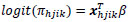
The survey logistic regression for a dichotomous dependent variable Yhji, i=1,...,nhj, j=1,...,nh, h=1,..., H, where h is the stratum, j is the cluster, and i is the household. Suppose that πhjik = P (Yhjik=1|Xhjik), is the probability of having diabetes. The survey logistic regression model is then expressed as:
 |
(2) |
An alternative formula for the survey logistic regression model can be written as:
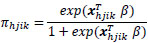 |
(3) |
where xhjik denote the matrix of explanatory variables and β denote the unknown vector of regression coefficients. Under a complex sampling design, the parameters β of the logistic regression model are estimated using the maximum pseudo-likelihood method [24]. This approach accounts for the sampling design and incorporates varying sampling weights into the estimation of β. PROC LOGISTIC and PROC SURVEYLOGISTIC in SAS 9.4 were employed to fit the standard logistic regression and survey logistic regression models.
3. RESULTS
In predicting the prevalence of diabetes in Kenyan men, Table 1 shows the significant interaction effects of age and health status, health status and hypertension, and health status and wealth index.
The interaction between age and self-reported health status shows that the relationship between age and diabetes is contingent on self-reported health status. That is, the men with “very bad” health status have a significant positive interaction (β = 0.1611, p-value = 0.0355), which means that the odds of diabetes rise more steeply with age in this group compared to those in “very good” health status. The odds ratio of 1.175 (95% CI: 1.011-1.365) implies that for each additional year of age, the risk of diabetes is elevated by approximately 17.5% among men with “very bad” health status. The interaction between age and health status suggests that the effect of age on diabetes varies by levels of self-reported health status.
The interaction between health status and hypertension reveals a highly significant and strong effect for men with “very bad” health status and hypertension (β = 14.6849, p-value < 0.0001). The estimated odds ratio is extremely high (2.4×10⁶), suggesting that the odds of having diabetes among men who self-report having “very bad” health and hypertension are astronomically higher compared to men with “very good” health status and no hypertension. This outcome suggests the combined risk of diabetes and comorbidity in men brings serious health issues.
| Effect | Estimate | SE | p-value | OR (95% CI) |
|---|---|---|---|---|
| Main effect | ||||
| Intercept | -9.5571 | 0.9413 | <.0001 | 7.07E-5 (1.12E-5; 0.0004) |
| Age | 0.0604 | 0.0132 | <.0001 | 1.062 (1.035; 1.090) |
| Alcohol consumption in the past month (ref= Non consumers of alcohol) | ||||
| Did not have even one drink | 0.2813 | 0.3872 | 0.4676 | 1.325 (0.620; 2.830) |
| Consume alcohol (but not every day) | -0.2229 | 0.2932 | 0.4471 | 0.800 (0.450; 1.422) |
| Every day/almost every day | 0.7793 | 0.6022 | 0.1958 | 2.180 (0.670; 7.097) |
| Educational level (ref= No education) | ||||
| Primary | 0.3371 | 0.6044 | 0.5770 | 1.401 (0.429; 4.580) |
| Secondary | 0.3770 | 0.6212 | 0.5440 | 1.458 (0.431; 4.925) |
| Higher | 0.6029 | 0.6394 | 0.3458 | 1.827 (0.522; 6.398) |
| Health status (ref= Very good) | ||||
| Very bad | 3.0260 | 0.6576 | <.0001 | 20.614 (5.681; 74.801) |
| Bad | 1.5131 | 0.7707 | 0.0498 | 4.541 (1.003; 20.567) |
| Moderate | 1.6605 | 0.3847 | <.0001 | 5.262 (2.475; 11.185) |
| Good | 0.4681 | 0.3400 | 0.1688 | 1.597 (0.820; 3.110) |
| Hypertension (ref= No) | ||||
| Yes | 2.2532 | 0.2847 | <.0001 | 9.518 (5.448; 16.629) |
| Marital status (ref= Never in union) | ||||
| Divorced | -0.9638 | 0.9192 | 0.2946 | 0.381 (0.063; 2.312) |
| Living with partner | 0.6037 | 0.5467 | 0.2696 | 1.829 (0.626; 5.340) |
| Married | 0.1549 | 0.3761 | 0.6804 | 1.168 (0.559; 2.440) |
| No longer living together/separated | -0.4352 | 0.7042 | 0.5367 | 0.647 (0.163; 2.573) |
| Occupation (ref= Not working) | ||||
| Agriculture-employee | 1.0631 | 0.6165 | 0.0848 | 2.895 (0.865; 9.694) |
| Agriculture-self employed | 0.4288 | 0.7136 | 0.5480 | 1.535 (0.379; 6.218) |
| Clerical | 1.4574 | 0.8308 | 0.0796 | 4.295 (0.843; 21.882) |
| Household and domestic | -0.6409 | 1.1881 | 0.5896 | 0.527 (0.051; 5.407) |
| Other | 1.9568 | 0.7394 | 0.0082 | 7.076 (1.661; 30.147) |
| Professional/technical/managerial | 0.6755 | 0.6454 | 0.2954 | 1.965 (0.55; 6.962) |
| Sales | 1.3154 | 0.6741 | 0.0512 | 3.726 (0.994; 13.966) |
| Services | 1.0682 | 0.7118 | 0.1336 | 2.910 (0.721; 11.743) |
| Skilled manual | 0.2059 | 0.6657 | 0.7571 | 1.229 (0.333; 4.529) |
| Unskilled manual | -0.0612 | 0.7199 | 0.9322 | 0.941 (0.229; 3.856) |
| Wealth index (ref= Middle) | ||||
| Poorer | -0.7351 | 0.3828 | 0.0550 | 0.479 (0.226; 1.015) |
| Poorest | -0.9956 | 0.4473 | 0.0262 | 0.369 (0.154; 0.888) |
| Richer | 0.0998 | 0.3345 | 0.7655 | 1.105 (0.0574; 2.128) |
| Richest | 0.7610 | 0.3170 | 0.0165 | 2.140 (1.150; 3.984) |
| Province (ref= Nairobi) | ||||
| Central | 0.6629 | 0.5356 | 0.2160 | 1.940 (0.679; 5.544) |
| Coast | 0.0588 | 0.5859 | 0.9201 | 1.061 (0.336; 3.344) |
| Eastern | 0.2434 | 0.5676 | 0.6682 | 1.276 (0.419; 3.880) |
| North Eastern | 1.7357 | 0.6040 | 0.0041 | 5.673 (1.736; 18.533) |
| Nyanza | 0.8840 | 0.5483 | 0.1071 | 2.421 (0.826; 7.089) |
| Rift Valley | -0.0375 | 0.5282 | 0.9434 | 0.963 (0.342; 2.712) |
| Western | 0.5304 | 0.5715 | 0.3535 | 1.700 (0.554; 5.209) |
| Significant interaction effect | ||||
| Age and Health status (ref=Very good) | ||||
| Age and Health status (Very bad) | 0.1611 | 0.0766 | 0.0355 | 1.175 (1.011; 1.365) |
| Age and Health status (Bad) | -0.0891 | 0.0442 | 0.0443 | 0.915 (0.839; 0.998) |
| Age and Health status (Moderate) | -0.0406 | 0.0274 | 0.1392 | 0.960 (0.910; 1.013) |
| Age and Health status (Good) | 0.0232 | 0.0280 | 0.4080 | 1.023 (0.969; 1.081) |
| Health status (ref=Very good) and Hypertension (ref=No) | ||||
| Health status (Very bad) and Hypertension (Yes) | 14.6849 | 1.4366 | <.0001 | 2.4E6 (1.43E5; 3.99E8) |
| Health status (Bad) and Hypertension (Yes) | -1.5524 | 1.3049 | 0.2344 | 0.212 (0.016; 2.732) |
| Health status (Moderate) and Hypertension (Yes) | 0.5937 | 0.8629 | 0.4916 | 1.811 (0.334; 9.826) |
| Health status (Good) and Hypertension (Yes) | 0.6362 | 0.7786 | 0.4140 | 1.889 (0.411; 8.691) |
| Health status (ref= Very good) and Wealth index (ref= Middle) | ||||
| Health status (Very bad) and wealth index (Poorer) | -13.9143 | 1.2227 | <.0001 | 9.06E-7 (8.3E-8; 9.95E-6) |
| Health status (Very bad) and wealth index (Poorest) | -14.9367 | 1.4711 | <.0001 | 3.26E-7 (1.8E-8; 5.83E-6) |
| Health status (Very bad) and wealth index (Richer) | 0.5675 | 1.3617 | 0.6769 | 1.764 (0.122; 25.444) |
| Health status (Very bad) and wealth index (Richest) | -12.4449 | 1.5616 | <.0001 | 3.94E-6 (1.8E-7; 8.40E-5) |
| Health status (Bad) and wealth index (Poorer) | 12.6312 | 1.4385 | <.0001 | 3.06E5 (1.8E4; 5.13E6) |
| Health status (Bad) and wealth index (Poorest) | 14.8351 | 1.6437 | <.0001 | 2.77E6 (1.1E5; 6.95E7) |
| Health status (Bad) and wealth index (Richer) | 14.4431 | 1.1195 | <.0001 | 1.87E6 (2.1E5; 1.68E7) |
| Health status (Bad) and wealth index (Richest) | 15.4985 | 2.1916 | <.0001 | 5.38E6 (7.3E4; 3.95E8) |
| Health status (Moderate) and wealth index (Poorer) | 0.0112 | 1.0993 | 0.9919 | 1.011 (0.117; 8.7210) |
| Health status (Moderate) and wealth index (Poorest) | 0.6618 | 1.3273 | 0.6181 | 1.938 (0.144; 26.137) |
| Health status (Moderate) and wealth index (Richer) | 1.1708 | 1.0207 | 0.2515 | 3.225 (0.436; 23.840) |
| Health status (Moderate) and wealth index (Richest) | 4.5601 | 1.2648 | 0.0003 | 95.59 (8.014; 1140.31) |
| Health status (Good) and wealth index (Poorer) | -1.9539 | 0.9735 | 0.0449 | 0.142 (0.021; 0.955) |
| Health status (Good) and wealth index (Poorest) | -1.7248 | 1.2637 | 0.1725 | 0.178 (0.015; 2.121) |
| Health status (Good) and wealth index (Richer) | -1.3487 | 0.7663 | 0.0786 | 0.260 (0.058; 1.166) |
| Health status (Good) and wealth index (Richest) | 1.6537 | 1.0774 | 0.1250 | 5.226 (0.633; 43.176) |
The interaction between health status and wealth index reveals complex relationships. Notably, men with “very bad” health status in the poorer, poorest, and richest wealth categories show an odds ratio of approximately zero (β = -13.9143 to β = -14.9367, p-value < 0.0001), indicating that diabetes is almost non-existent in these groups compared to those men with reported health very good and wealth index middle. On the other hand, men with “bad” health status in the poorest and richest wealth categories exhibit significantly increased odds of diabetes (OR = 2.77×10⁶ and 1.87×10⁶, respectively), reflecting an extreme disparity in diabetes risk across wealth groups.
These findings highlight critical interactions in diabetes risk, particularly the compounding effects of poor health, hypertension, and socioeconomic status. The results suggest that targeted interventions should consider these interaction effects, emphasising age-specific strategies, hypertension management, and wealth disparities in health outcomes.
The findings from the survey logistic regression model reveal the relationship between the different risk factors and diabetes prevalence in men (Table 1). A significant predictor of diabetes was age (p-value < 0.0001) with an estimated coefficient of 0.0604. This indicates that the probability of having diabetes increases with an increase in age. The odds ratio (OR) of 1.062 (95% CI: 1.035-1.090) means that for each unit increase of age, the odds of having diabetes are increased by approximately 6.2%, holding all other factors constant.
The health status demonstrated a strong correlation with the prevalence of diabetes. In comparison with men who perceived their health as “very good”, those who answered “very bad” for their health indicate significantly higher odds of diabetes (OR = 20.614, 95% CI: 5.681- 74.801, p-value < 0.0001).
Similarly, the odds ratio for males who assessed their health as “bad” was 4.541 (95% CI: 1.003-20.567, p-value = 0.0498), while the odds ratio for men who rated their health as “moderate” was 5.262 (95% CI: 2.475-11.185, p-value < 0.0001). These findings suggest that men who report poorer health status have much higher odds of having diabetes. Men who reported having hypertension were significantly more likely to also have diabetes, making hypertension a powerful predictor (OR = 9.518, 95% CI: 5.448- 16.629, p-value < 0.0001). The strong relationship remained because of the established connection between hypertension and diabetes, which indicates common risk factors (comorbidities).
Compared to those who do not work, men in the “other” occupation category had significantly greater odds of having diabetes (OR = 7.076, 95% CI: 1.661-30.147, p-value = 0.0082). Additionally, the men in the sales category had an OR of 3.726 (95% CI: 0.994-13.966) and a marginally significant association (p-value = 0.0512). No other occupational category showed any significant association.
The wealth index showed variable effects, with the “Poorest” group showing significantly lower odds of diabetes compared to the “Middle” group (OR = 0.369, 95% CI: 0.154-0.888, p-value = 0.0262). Conversely, men in the “Richest” group showed significantly higher odds of diabetes compared to the middle wealth index group (OR = 2.140, 95% CI: 1.150-3.984, p-value = 0.0165). This result suggests a complex relationship between socioeconomic status and diabetes prevalence, with both extremes of the wealth index showing different risk exposures. As a summary, we can see that the poorest and the poorer wealth index groups show lower odds of diabetes than the middle wealth index group, while the richer and the richest wealth index groups show higher odds of diabetes than the middle wealth index group.
The province has a large effect on the prevalence of diabetes among the Kenyan male population. Specifically, the North Eastern province contributes to a statistically significant variation in the prevalence of diabetes compared to Nairobi (p-value = 0.0041). The odds ratio (OR) of 5.673 (95% CI: 1.736-18.533) shows that the odds of diabetes for men residing in the North Eastern province are over 5.6 times that of men in Nairobi, after adjusting for other factors in the model. The implication is that the prevalence of diabetes among men in North Eastern Kenya is higher relative to men in Nairobi, even though Nairobi has a high degree of urbanisation. This result underscores the need for diabetes interventions at a provincial level for the North Eastern province, where management specifically tailored to education programmes and screening programmes could be implemented to alleviate the diabetes burden.
Fig. (1) shows that the impact of health status on diabetes is modified by hypertension status. The predicted diabetes probability decreases as health status improves for both men with and without hypertension, but is more pronounced for men with hypertension. The probability of developing diabetes varies depending on hypertension status. Hypertension increases diabetes risk, with health improvements having a greater impact on reducing diabetes probability in hypertensive men. The predicted probability of diabetes in males without hypertension does not vary significantly. Across males with varying health statuses, it remains rather stable.
Fig. (2) shows that men with poor health, particularly in middle and richer wealth groups, have higher diabetes probabilities. The interaction between health status and wealth index is significant, with poor health status associated with higher diabetes risk in middle and richer wealth groups. Wealthier men with poor health are at a higher risk of diabetes, indicating that wealth alone does not guarantee protection against it.
Table 2 displays the results of the two models, the fitted standard logistic regression and survey logistic regression models. A significant positive effect of age on diabetes was observed in both models (p-value < 0.0001), indicating that the likelihood of having diabetes increases with age. Health status also played a critical role, with men reporting very bad health experiencing significantly higher odds of diabetes. The survey logistic regression estimated an effect of 3.0260 (p-value < 0.0001), while the standard logistic regression provided an estimate of 2.6611 (p-value = 0.0007). Similarly, bad health was significantly associated with increased diabetes risk (β = 1.5131, p-value = 0.0498 in the survey model and β = 1.1829, p-value = 0.0303 in the logistic regression model), while moderate health was also a significant predictor, but good health did not show a significant effect. Hypertension was strongly associated with diabetes in both models (p-value < 0.0001), with estimates of 2.2532 (survey logistic regression) and 1.9115 (logistic regression), confirming a higher risk of diabetes among hypertensive men.
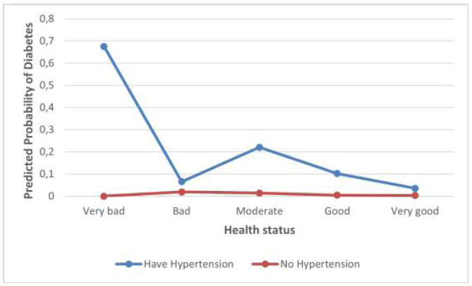
Interaction effect between health status and hypertension.
Occupation was also significant, with clerical workers, sales workers, and those in “other” professions having higher odds of diabetes in both models. The survey logistic regression model indicated that “other” occupations had a stronger effect (β = 1.9568, p-value = 0.0082) than the standard model (β = 1.3271, p-value = 0.0310). Sales work was significant in the logistic regression model (β = 1.2047, p-value = 0.0184) and nearly significant in the survey model (β = 1.3154, p-value = 0.0512). The wealth index also revealed disparities, with the poorest men having significantly lower odds of diabetes compared to those in the middle wealth group (p-value < 0.05), whereas the richest men had significantly higher odds (β = 0.7610, p-value = 0.0165) in the survey model and β = 0.6470, p-value = 0.0284 in the standard model). Geographical disparities were evident, as men in the North Eastern province had significantly higher odds of diabetes (p-value < 0.01) in both models. The interaction effects indicated a significant relationship between health status and wealth index in both models, especially among men with poor health and varying wealth levels.
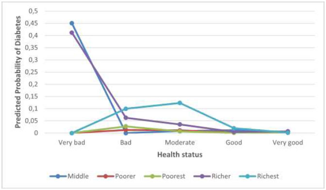
Interaction effect between health status and wealth index.
| Effect | Survey Logistic Regression | Logistic Regression | ||||
|---|---|---|---|---|---|---|
| Estimate | SE | p-value | Estimate | SE | p-value | |
| Main Effect | ||||||
| Intercept | -9.5571 | 0.9413 | <.0001 | -8.2109 | 0.8583 | <.0001 |
| Age | 0.0604 | 0.0132 | <.0001 | 0.0558 | 0.0117 | <.0001 |
| Alcohol in the past month (ref= Non consumers of alcohol) | ||||||
| Did not have even one drink | 0.2813 | 0.3872 | 0.4676 | 0.3520 | 0.2468 | 0.1538 |
| Consume alcohol (but not every day) | -0.2229 | 0.2932 | 0.4471 | -0.1157 | 0.2320 | 0.6180 |
| Every day/almost every day | 0.7793 | 0.6022 | 0.1958 | 0.4529 | 0.5675 | 0.9522 |
| Educational level (ref= No education) | ||||||
| Primary | 0.3371 | 0.6044 | 0.5770 | -0.2307 | 0.4551 | 0.6121 |
| Secondary | 0.3770 | 0.6212 | 0.5440 | 0.0059 | 0.4621 | 0.9898 |
| Higher | 0.6029 | 0.6394 | 0.3458 | -0.0296 | 0.4929 | 0.9522 |
| Health status (ref= Very good) | ||||||
| Very bad | 3.0260 | 0.6576 | <.0001 | 2.6611 | 0.7866 | 0.0007 |
| Bad | 1.5131 | 0.7707 | 0.0498 | 1.1829 | 0.5461 | 0.0303 |
| Moderate | 1.6605 | 0.3847 | <.0001 | 1.1749 | 0.2577 | <.0001 |
| Good | 0.4681 | 0.3400 | 0.1688 | 0.1239 | 0.2421 | 0.6088 |
| Hypertension (ref= No) | ||||||
| Yes | 2.2532 | 0.2847 | <.0001 | 1.9115 | 0.2098 | <.0001 |
| Marital status (ref= Never in union) | ||||||
| Divorced | -0.9638 | 0.9192 | 0.2946 | -0.2827 | 0.8038 | 0.7250 |
| Living with partner | 0.6037 | 0.5467 | 0.2696 | 0.5467 | 0.4800 | 0.2547 |
| Married | 0.1549 | 0.3761 | 0.6804 | 0.1442 | 0.3371 | 0.6687 |
| No longer living together/separated | -0.4352 | 0.7042 | 0.5367 | -0.7737 | 0.6620 | 0.2425 |
| Occupation (ref= Not working) | ||||||
| Agriculture-employee | 1.0631 | 0.6165 | 0.0848 | 0.7906 | 0.4674 | 0.0907 |
| Agriculture-self employed | 0.4288 | 0.7136 | 0.5480 | 0.9654 | 0.6762 | 0.1534 |
| Clerical | 1.4574 | 0.8308 | 0.0796 | 1.4608 | 0.7165 | 0.0415 |
| Household and domestic | -0.6409 | 1.1881 | 0.5896 | -0.3477 | 1.0915 | 0.7501 |
| Other | 1.9568 | 0.7394 | 0.0082 | 1.3271 | 0.6153 | 0.0310 |
| Professional/technical/managerial | 0.6755 | 0.6454 | 0.2954 | 0.5434 | 0.4930 | 0.2703 |
| Sales | 1.3154 | 0.6741 | 0.0512 | 1.2047 | 0.5111 | 0.0184 |
| Services | 1.0682 | 0.7118 | 0.1336 | 0.8595 | 0.5896 | 0.1449 |
| Skilled manual | 0.2059 | 0.6657 | 0.7571 | 0.4051 | 0.4920 | 0.4102 |
| Unskilled manual | -0.0612 | 0.7199 | 0.9322 | 0.2649 | 0.5488 | 0.6293 |
| Wealth index (ref= Middle) | ||||||
| Poorer | -0.7351 | 0.3828 | 0.0550 | -0.3017 | 0.3212 | 0.3475 |
| Poorest | -0.9956 | 0.4473 | 0.0262 | -0.7867 | 0.3841 | 0.0405 |
| Richer | 0.0998 | 0.3345 | 0.7655 | 0.3650 | 0.2703 | 0.1770 |
| Richest | 0.7610 | 0.3170 | 0.0165 | 0.6470 | 0.2952 | 0.0284 |
| Province (ref= Nairobi) | ||||||
| Central | 0.6629 | 0.5356 | 0.2160 | 0.3131 | 0.5368 | 0.5597 |
| Coast | 0.0588 | 0.5859 | 0.9201 | 0.1382 | 0.5510 | 0.8019 |
| Eastern | 0.2434 | 0.5676 | 0.6682 | 0.0174 | 0.5453 | 0.9746 |
| North Eastern | 1.7357 | 0.6040 | 0.0041 | 1.5879 | 0.6034 | 0.0085 |
| Nyanza | 0.8840 | 0.5483 | 0.1071 | 0.4917 | 0.5332 | 0.3564 |
| Rift Valley | -0.0375 | 0.5282 | 0.9434 | -0.0639 | 0.5227 | 0.9027 |
| Western | 0.5304 | 0.5715 | 0.3535 | 0.2878 | 0.5694 | 0.6132 |
| Significant interaction effects in both models | ||||||
| Health status (ref= Very good) and Wealth index (ref= Middle) | ||||||
| Health status (Very bad) and wealth index (Poorer) | -13.9143 | 1.2227 | <.0001 | -14.1432 | 1888.2 | 0.9940 |
| Health status (Very bad) and wealth index (Poorest) | -14.9367 | 1.4711 | <.0001 | -14.7366 | 1014.3 | 0.9884 |
| Health status (Very bad) and wealth index (Richer) | 0.5675 | 1.3617 | 0.6769 | -0.9024 | 2.1045 | 0.6681 |
| Health status (Very bad) and wealth index (Richest) | -12.4449 | 1.5616 | <.0001 | -13.8299 | 1595.8 | 0.9931 |
| Health status (Bad) and wealth index (Poorer) | 12.6312 | 1.4385 | <.0001 | 13.0124 | 735.6 | 0.9859 |
| Health status (Bad) and wealth index (Poorest) | 14.8351 | 1.6437 | <.0001 | 14.1770 | 735.6 | 0.9846 |
| Health status (Bad) and wealth index (Richer) | 14.4431 | 1.1195 | <.0001 | 14.0249 | 735.6 | 0.9848 |
| Health status (Bad) and wealth index (Richest) | 15.4985 | 2.1916 | <.0001 | 15.2222 | 735.6 | 0.9835 |
| Health status (Moderate) and wealth index (Poorer) | 0.0112 | 1.0993 | 0.9919 | 0.7750 | 0.9386 | 0.4090 |
| Health status (Moderate) and wealth index (Poorest) | 0.6618 | 1.3273 | 0.6181 | 1.2278 | 1.0553 | 0.2446 |
| Health status (Moderate) and wealth index (Richer) | 1.1708 | 1.0207 | 0.2515 | 0.8170 | 0.8495 | 0.3362 |
| Health status (Moderate) and wealth index (Richest) | 4.5601 | 1.2648 | 0.0003 | 3.5002 | 1.0673 | 0.0010 |
| Health status (Good) and wealth index (Poorer) | -1.9539 | 0.9735 | 0.0449 | -1.7021 | 0.8988 | 0.0583 |
| Health status (Good) and wealth index (Poorest) | -1.7248 | 1.2637 | 0.1725 | -1.3048 | 0.9717 | 0.1793 |
| Health status (Good) and wealth index (Richer) | -1.3487 | 0.7663 | 0.0786 | -1.6150 | 0.6719 | 0.0162 |
| Health status (Good) and wealth index (Richest) | 1.6537 | 1.0774 | 0.1250 | 0.8917 | 0.9117 | 0.3281 |
| Model evaluation | |||
|---|---|---|---|
| Overall significance | Chi-square | D.F | p-value |
| Likelihood Ratio | 490.5174 | 37 | <.0001 |
| Score | 533.9672 | 37 | <.0001 |
| Wald | 376.1103 | 37 | <.0001 |
| NOTE: First-order Rao-Scott design correction 0.9973 is applied to the likelihood ratio test. | |||
| Association of Predicted Probabilities and Observed Responses | |||
| Percent Concordant | 79.6 | Somers’D | 0.665 |
| Percent Discordant | 13.1 | Gamma | 0.718 |
| Percent Tied | 7.4 | Tau-a | 0.013 |
| Pairs | 2003820 | c | 0.833 |
The interaction between very bad health and poorer wealth index was significant in the survey logistic regression (β = -13.9143, p-value < 0.0001) but not in the logistic regression model (β = -14.1432, p-value = 0.9940). Similarly, men in the poorest wealth group with very bad health had significantly lower odds of diabetes in the survey model (β = -14.9367, p-value < 0.0001), while the standard model did not detect significance (β = -14.7366, p-value = 0.9884). Those with bad health in the richest wealth category were at much higher risk of diabetes, as shown by a strong positive interaction in the survey logistic regression (β = 15.4985, p-value < 0.0001) and logistic regression (β = 15.2222, p-value = 0.9835). Moderate health and the richest wealth index were also significantly associated with diabetes (β = 4.5601, p-value = 0.0003 in the survey model and β = 0.0010 in the logistic regression model). A notable negative interaction was found in the logistic regression model for good health and a richer wealth index (β = -1.6150, p-value = 0.0162), suggesting that wealthier men with good health had lower odds of diabetes. Comparing the models, the survey logistic regression, which accounts for the complex survey design, resulted in different standard errors and slightly adjusted estimates compared to the standard logistic regression. Some effects were significant in the survey model but not in the standard model, likely due to the latter underestimating standard errors for interaction terms. These findings suggest that the survey logistic model is preferable when working with population-weighted data, offering more reliable estimates for policy-related decisions. The strong interaction between health status and wealth index highlights the critical role of socio-economic disparities in diabetes prevalence.
4. DISCUSSION
At the 5% significance level, the Wald, Score, and Likelihood Ratio tests all show statistical significance (Table 3). These suggest that the covariates notably impact the probability of developing diabetes. According to Table 3, 83.3% of the predictions are correct, reflecting a strong correlation between the observed outcomes and the predicted probabilities. Gamma, Somers’ D, and concordance values are 71.8%, 66.5%, and 79.6%, respectively.
5. STUDY LIMITATIONS
This study used secondary data from the 2022 Kenya Demographic and Health Survey (KDHS). As the secondary data, the variables available for analysis were limited to those collected in the DHS, restricting the inclusion of potentially unmeasured risk factors. For example, variables like family history of diabetes and physical activity, which are regarded as risk factors associated with diabetes in some studies, are not included in DHS data. Certain variables (e.g., alcohol consumption, health status) may introduce recall bias. The data represents a snapshot in 2022 and may not reflect trends or changes in diabetes prevalence over time. Future studies should consider longitudinal designs and make use of clinical data to expand the knowledge of diabetes dynamics among Kenyan men.
CONCLUSION
To develop strategies for reducing the risk of diabetes, policymakers must focus on the important determinants. According to this study, the risk of diabetes can be decreased by enhancing health by addressing chronic conditions, like hypertension. Diabetes prevalence can be reduced by addressing age-related risk factors and putting preventive programmes for senior citizens into place. Enhancing healthcare access for individuals in poor wealth categories while promoting awareness among wealthier individuals about diabetes risk factors is crucial. Targeted interventions for older men and those in lower wealth quintiles should focus on increasing access to affordable screening and community-based education programs that promote healthy lifestyles. Culturally tailored campaigns emphasising diet, physical activity, and routine check-ups can help address both knowledge gaps and financial barriers, ultimately reducing diabetes risk in these high-vulnerability groups. Additionally, focusing on occupational groups with higher diabetes risk, such as those in clerical, sales, and other sectors, can aid in targeted intervention efforts. The government of Kenya needs to implement programmes targeted at regions such as the North Eastern Province, where diabetes prevalence is significantly higher, to develop strategies for reducing the burden of diabetes in these areas. In summary, the study makes an important contribution by identifying key risk factors for diabetes among men in Kenya using nationally representative data. Future research could expand on these findings by incorporating behavioural, genetic, and environmental factors to construct a more comprehensive and holistic risk profile for diabetes.
AUTHORS’ CONTRIBUTIONS
The authors confirm contribution to the paper as follows: D.T.-L.N.: Conceptualisation, Visualisation, Methodology, Software, Data curation, Writing – original draft, Writing – review & editing; S.F.M.: Validation, Supervision, Resources, Writing – review & editing;. All authors reviewed the results and approved the final version of the manuscript.
LIST OF ABBREVIATIONS
| KDHS | = Kenya Demographic and Health Survey |
| KNBS | = Kenya National Bureau of Statistics |
| MoH | = Ministry of Health |
| K-HMSF | = Kenya Household Master Sample Frame |
| EAs | = Enumeration Areas |
| NCDs | = Non-communicable Diseases |
| T1DM | = Type 1 Diabetes Mellitus |
| T2DM | = Type 2 Diabetes Mellitus |
| GDM | = Gestational Diabetes Mellitus |
ETHICS APPROVAL AND CONSENT TO PARTICIPATE
Ethical approval for the original data collection was granted by the Kenya Medical Research Institute (KEMRI) Ethics Review Committee, affiliated with KEMRI, Kenya. The DHS survey protocol was reviewed and approved by the ICF Institutional Review Board in the United States as well. The publicly available dataset contains no personally identifiable information, and all geographic identifiers are anonymised. Since the analysis involved secondary data with no direct contact with human subjects, additional ethical approval was not required for this specific study.
HUMAN AND ANIMAL RIGHTS
All human research procedures followed were in accordance with the ethical standards of the committee responsible for human experimentation (institutional and national), and with the Helsinki Declaration of 1975, as revised in 2013.
AVAILABILITY OF DATA AND MATERIALS
The data for this study were requested from DHS (Demographic Health Surveys) and it is available on their website: https://www.dhsprogram.com/.
FUNDING
This work was supported by Aspen Pharmacare. Aspen is a global specialty and branded pharmaceutical company, improving the health of patients across the world through its high quality and affordable medicines.
CONFLICT OF INTEREST
Dr. Sileshi Fanta Melesse is the Editorial Advisory Board member of the Open Public Health Journal.
ACKNOWLEDGEMENTS
The author acknowledges Professor SM for the support he has been offering. The Authors are grateful for the data that they have been provided by DHS.