All published articles of this journal are available on ScienceDirect.

A Bayesian Hierarchical Analysis of Geographical Patterns for Child Mortality in Nigeria
Abstract
Background:
In an epidemiological study, disease mapping models are commonly used to estimate the spatial (or temporal) patterns in disease risk and to identify high-risk clusters, allowing for health interventions and allocation of the resources. The present study proposes a hierarchical Bayesian modeling approach to simultaneously capture the over-dispersion due to the effect of varying population sizes across the districts (regions), and the spatial auto-correlation inherent in the childhood mortality at districts (state) level in Nigeria.
Methods:
This cross-sectional study was based on 31842 children data extracted from the 2013 Nigeria Demographic and Health Survey (DHS). Of these children, 2886 died before reaching the age of five years. A Standardized Mortality Ratio (SMR) was estimated for each district (state) and mapped to highlight the risk patterns and detect an unusual low (high) clusters relative risk of childhood mortality. Generalized Poisson regression models were formulated with random effects to estimate the mortality risk and then explored to investigate the relationship of under-five child mortality and the regional risk factors. The random effects are formulated to reflect the potential tendency of “neighbouring” regions to have similar risk patterns and the spatial heterogeneity effect was used to capture geographical inequalities in the mortality outcomes. The models were implemented using a full Bayesian framework. All model parameters were estimated in WinBUGS via Markov Chain Monte Carlos (MCMC) simulation techniques.
Results:
The results showed that of the economically deprived households, 2.088: 95% CI (1.088, 3.165) were significantly associated with childhood mortality, while unhygienic sanitation and lack of access to improved water sources were positively associated with child mortality, but not statistically significant at 5% probability level. The geographical variation of the under-five mortality prevalence was found to be attributed to 69% clustering and 31% was due to spatial heterogeneity factors. The predicted probability maps identified clusters of high risk mortality in the northern regions and low prevalence of concentrated mortality in the south-west regions of Nigeria.
Conclusion:
The results demonstrated the flexibility of the approach that explored the geographical variation in the potential risk factors of child mortality and that it provides a better understanding of the regional variations of mortality risks. Nonetheless, both representations can help to provide information for the initiation of public health interventions.
1. INTRODUCTION
Despite remarkable growth recorded by many economies in the last two decades, many developing countries have failed to attain the target Millennium Development Goals (MDGs 1) four(4), the (reduction of under-five mortality by two-thirds between 1990 and 2015) and seven (7), the targets for water and sanitation in urban. Five countries accounted for half of the global infant mortality with Nigeria being the third largest contributor to the under- five mortality rate among children in sub-Saharan Africa [1, 2]. In 2013, the mortality rates for the five countries were: India (24%), Pakistan (10%), Nigeria (9%), the Democratic Republic of Congo (DRC) (4%) and Ethiopia (3%) as reported in [3]. According to a UNICEF/World Bank report, the prevalence of high child mortality in Africa is concentrated in the four sub-Saharan countries of Malawi, Nigeria, Tanzania and Zambia. In 2003, the mortality rates among children less than five years old were estimated at 187 per 1000 live births for Malawi, 183 for Nigeria, 165 for Tanzania, and 202 for Zambia, which are among the highest in the world [4].
Globally, about a billion people still lack access to improved drinking water and approximately 2.5 billion lack improved toilet facilities, which are major causes of diarrhoea infections, as reported in [5, 6]. Unimproved hygiene during food preparation, contaminated water, open defecation and improper faeces disposal could also result in diarrhoea among children, which globally accounts for approximately 1.4 million child deaths each year [6, 7]. In a study recently conducted by Black et al. [8], it was reported that an estimated 8.8 million children died worldwide from infectious diseases and about 68% (5.970 million) death was caused by diarrhoea. However, Aiello et al. [9], previously reported that access to improved water and sanitation can lead to a reduction in cases of child diarrhoea and childhood mortality rates.
The major contributory cause of child mortality is attributed to individual family poverty levels or poor household’s environments, highly concentrated in rural areas or slums in big cities [10, 11]. The household poverty and poor environments could exacerbate the problems of poor health and disease prevalence among children, and hence, the high mortality risks. It has been suggested that health inequalities not only reflect the poor health of the most disadvantaged people, but also the apparently limitless health benefits associated with rising socioeconomic status [7, 12].
A good number of studies have investigated the health inequality of sub- populations from the perspective of geography, epidemiology, and public health showing that where people live significantly affects their health outcomes are well detailed in the literature [13, 14]. Some studies commonly employ disease mapping models and applications. A wide range of these studies include Sudden Infant Death syndrome (SID) by [15], lip cancer in Scotland by [16], child mortality by [17], and stomach and bladder cancers in Missouri by [18]. Other studies have found significant associations between proximity to industrial sites and leukemia and lymphoma as reported in [19]. Recently, a study conducted by [20] on congenital anomalies and total cancer mortality has shown that the diseases were found to be associated with waste-related environmental pollution.
The challenge of the geographical analysis of health is that it has to deal with methodological uncertainties as well as social and political issues. Methodological uncertainties are caused by issues of ecological fallacy, scale, Modifiable Areal Unit Problems (MAUP) and spatial autocorrelation [21, 22]. The problems can be inherent in making inference about sub-population or area characteristics as individual within the population. The statistical issues with disease mapping models involve small area estimations of aggregated data over small area requiring taking into account local spatial correlation [23, 24], who states that data sparseness is a major problem in small area analysis, especially when it involves rare diseases. A small number of observed and expected disease occurrences at health unit, district or regional level can lead to unstable risk estimates or unusual relative risk estimates [25]. To handle the problem of over-dispersion and sparsity, random effect models are commonly introduced into the models to deal with the problems arising from high varying population sizes of areas with count data, which are spatially aggregated over regions as suggested in several studies [26-28].
This study therefore used an exploratory method to estimate the SMR of each state (district) in Nigeria and mapped it onto the geographical regions to highlight unusual clusters of low (high) child mortality in the country. The study then proposed Bayesian hierarchical models to capture the un- measured random heterogeneity effects in child mortality data and estimated the geographical inequalities of the under-five mortality prevalence across the districts (states). The statistical inference was performed within a full Bayesian framework.
The paper is structured in the following order. Section 1 provides the background of the study relating to environmental risk factors of child mortality. In Section 2, the study discusses the study design and data collection procedure, and the disease mapping models, including exploratory data analysis. Section 3 described the Bayesian hierarchical models within generalized linear mixed models. In Section 4, the proposed models are applied to under-five mortality rates from the 2013 Nigeria DHS. Section 5 presents the discussion and the concluding remarks of the present study.
2. MATERIALS AND METHODS
2.1. The Data Exploration
The common sources of data for cause-specific mortality include vital registration systems, sample registration systems, nationally representative household surveys and sentinel Demographic Surveillance Sites (DSS) for epidemiological studies. With an exception of a few countries, such as South Africa, reliable and functioning vital registration systems have been presented a challenge in supporting attribution of causes of child death in many low-middle income countries, particularly in sub- Saharan Africa [29, 30].
The main source of data for researchers to guide policy makers in a developing country such as Nigeria is the National DHS conducted by the Data Measure program. The United States Agency for International Development (USAID) has provided the technical assistance and funding to conduct surveys in several developing countries, thereby promoting global understanding of public health. The DHS program collects survey data nationally on a variety of socio-demographic and health related issues. The survey collected information about the background of the respondents, specifically collected information on fertility levels, marriage, fertility preference, awareness and use of family planning methods, child mortality and child nutrition. Detailed information and procedures about the data collection, and questionnaires have been published elsewhere by [31].
The 2013 NDHS survey conducted by the DHS measure used a multi-stage cluster design consisting of 40,320 households in 904 clusters with 372 in urban areas and 532 in

rural areas. The survey successfully interviewed 38,948 women occupied in 38, 520 households nested in 886 clusters. This yielded a household response rate for women of 99%. Data extracted from the 2013 NDHS for the present study are: the number of children born between 2008 and 2013, the number of children alive and counts of child deaths at the time of the survey, the proportion of poorest and poor households, the number of cases (children) experiencing diarrhoea two weeks prior to the survey, the number of households using solid cooking fuels such as, coal, charcoal, fire wood, cow dung and agricultural crop residues.
For the purpose of the present study, Fig. (1) shows the geographical map of Nigeria showing 36 states (districts) and the Federal Capital Territory, Abuja. Nigeria comprises of six geopolitical regions; North-East, North-West, North-Central, South-East, South-South, and South-West which are sub-divided into 36 administrative states and the Federal Capital Territory (FCT). The population groupings within the geopolitical regions and states are relatively homogeneous. Also, the people's cultural beliefs such as the demographic characteristics, arid environment factors and socio-cultural structures are considered similar within the geopolitical zones and states.
In disease mapping, the first step is the removal of the effect of the confounding factors on the risk estimate in the study population through distribution standardization. Standardization of mortality rates or disease incidence is a basic tool in both demography [32] and epidemiology [33, 34]. The most frequently used method in epidemiology is the traditional method for estimating the relative risk is the internal standardization method, which calculates the expected disease counts as functions of the observed numbers of cases. However, such models are regarded as incoherent and not generative probabilistically according to [35], because the observed count appears on both sides of the equation.
Consider the death counts, Yk aggregated data over a state (district), say, 37 (k = 1;::: ; 37) states, where the mother, k resides in Nigeria. In this study, the SMR is calculated as
 |
(1) |
and
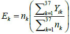 |
In equation (1), Yk is a random variable representing the number of observed cases (under-five deaths) in each kth state(district) and nk represents the number of children at risk (number of under-five children in each state, k). In addition SMRk is calculated as the ratio of observed number of child death cases to the expected number of cases in the kth state, representing the risk of each kth area (state). Whenever the value of SMR is greater (lower) than one (1), it indicates that the area (state) k has a higher (lower) risk than the average disease risk of the whole region. For example, for SMRk, it can be said that area k has a 25% higher risk of the disease (childhood morbidity). These quantities SMR are plotted as a crude map. This estimator is unbiased, and is frequently used by epidemiologists. However, this estimate is based only on a sample size of one and hence it is not really statistically useful because it is a saturated model. Some of the advantages and disadvantages of a crude map of the SMR have been highlighted by Lawson et al. [15].
In recent years, the attempts to map incidence and mortality from diseases such as cancer have been explored. Such maps usually display either relative rates in each district or province, as measured by a SMR or similar index. The standard models are detailed in the literature on the empirical methods and its applications can be found in [36, 37]. Clayton [38] has earlier provided approach for estimating the SMR using Bayesian methodology. According to [26] the mean of the estimator,
 k and its variance, which will be large if the expected number of incidence cases is small. This is one of the disadvantages of using the SMR. Other disadvantages are discussed by [39], showing that the SMR is based on a ratio estimator.
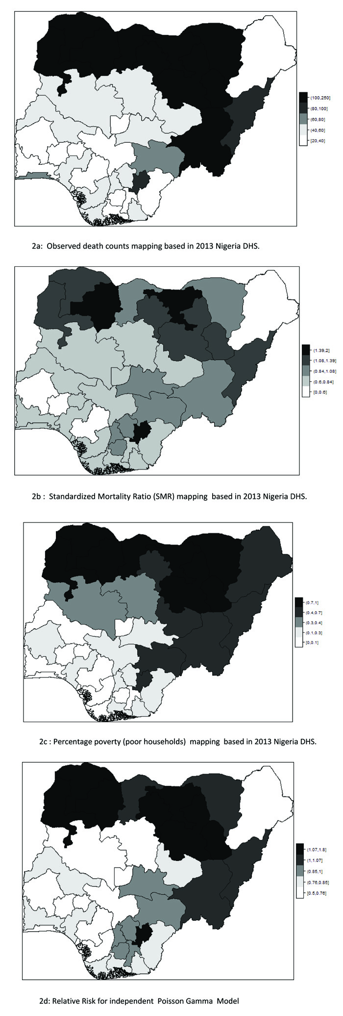
From Fig. (2a), (the raw death counts map), a cluster of child mortality was occurred and concentrated in the northern part of Nigeria. With reference to Fig. (2c), most northern states are darker than the southern regions. This indicates that there are more economically deprived households in northern Nigeria than in the southern regions. Reference to Fig. (2b) , in (SMR), shows few states with an unusual low or (high) mortality incidence, while such districts (states) are bordered /surrounded by relatively high counts. For instance, the observed (isolated) low incidence of mortality in Borno State, which is surrounded by states with relatively high death counts, is an evidence of geographical disparities with no clear patterns. Another scenario can be seen in a state like Zamfara (with a high mortality count (130)), which shares boundaries with states in the north -western region with relative high mortality risk states such as Kebbi (109.55) and Sokoto (124.77). These scenarios may better be handled by a spatial random effect model or the BYM model, which exhibit borrowing strength that is regions close to each other share similarities in their prevalence.
Fig. (1a) Displays the map of observed mortality counts across the 37 states(districts) in Nigeria, Fig. (2b) is the map of SMRs of the child mortality and corresponding Table 1 with SMRs that vary widely around their mean, 0.920, (standard deviation: 0.306). Although, the evidence of observed lower SMRs were recorded in the southern regions of the country, the geographic variation in child mortality with clustering of high mortality observed in the northern states with a relatively low mortality prevalence (isolated area) of Borno state is apparent. No clear spatial pattern emerges from the map.
Fig. (1b) also depicts the empirical estimation of SMR of child mortality. The geographical patterns of child mortality distribution are similar for Fig. (1a), raw mortality count map and the crude SMR 2(b). The clusters of high mortality or concentrated mortality found in the northern regions can be attributed to partly unobserved heterogeneity and environmental factors. The smooth SMR map (d) shows evidence of localized spatial smoothness and neighbouring states exhibited similar patterns of mortality risk, while other neighbouring regions far apart showed different (local) risks patherns. In Figs. (2b and 2d), regions coloured black show the SMRs with RR greater than one indicates significantly excess(higher) mortality . The light coloured regions are states signify low prevalence (RR less than one) of child mortality, while the grey coloured regions are not significant.
The map of Relative Risk (RR mean) from the independent Poisson model is shown in Fig. ( 2d). The map depicts that the model could not capture the geographical variation in the spatial pattern of the actual mortality count data.
For instance, discontinuities can be seen in some states with clustering of high mortality rates in the north when compared with the observed counts map. Katsina State recorded the highest expected counts and posterior mean RR, but the Poisson model (no random effect) would classify Katsina lower than the actual mortality level. Another scenario in the spatial disparities was also observed in Ekiti State in south-west Nigeria with small expected counts, but the state was an elevated high risk. This dispersion can be attributed to small population size. The independent Poisson sometimes under-estimates the mortality risk such as Balyesa and Lagos, perhaps these could result from a high expected value (denominator).
A careful inspection of the expected counts in Fig. (2) reveals that higher child mortality risk were detected in some states of the north regions resulting from empirical computation of SMR i.e. Kano, due to large expected count of 197.827 (divisor)(refer to Table 2). Four other states were considered with expected counts of 46.569, 51.153, 61.420 and 131.64 corresponding to approximate percentile values of 10th, 25th, 50th and 90th of the expected counts respectively. It is worth mentioning that the choice of unusually low relative risk values (SMR) (10th percentile of the expected counts) would establih an epidemiological importance. Interestingly, some districts (states) had unusual low death rates surrounded by neighbouring states with a fairly high mortality risk. The expected mortality rates of the four states correspond to the percentiles (10th - 90th percentile): Abia (46.57), Osun (51.12), Plateau Sate (61.42) and Jigawa (131.64). For example, Plateau state (61.42) had relative low prevalence but is surrounded by states had relatively high mortality. In such cases, the mortality rates in those neighbouring states may have a substantial influence on the smoothing effects on states that share borders. This scenario can be handled by the spatial Conditional Auto-Regressive (CAR) model.
| Minimum | 1st Quartile | Median | Mean | 3rd Quartile | Maximum | |
|---|---|---|---|---|---|---|
| Observed counts (y) | 21 | 39 | 51 | 78 | 104 | 229 |
| Expected Counts (E) | 43.73 | 51.15 | 61.42 | 78.00 | 98.64 | 197.80 |
| SMR | 0.4105 | 0.7251 | 0.8303 | 0.9197 | 1.0770 | 1.7570 |
| State | Observed Deaths(O) | Expected Count(E) | Relative Frequency | SMR | Total Birth(N) |
|---|---|---|---|---|---|
| Abia | 39 | 46.57 | 1.35 | 0.425 | 508 |
| Adamawa | 100 | 91.76 | 3.47 | 1.894 | 1001 |
| Akwa Ibom | 43 | 52.80 | 1.49 | 0.873 | 576 |
| Anambra | 46 | 49.23 | 1.59 | 0.349 | 537 |
| Bauchi | 180 | 131.92 | 6.24 | 2.392 | 1439 |
| Bayelsa | 58 | 75.26 | 2.01 | 0.959 | 821 |
| Benue | 61 | 60.50 | 2.11 | 1.109 | 660 |
| Borno | 28 | 55.00 | 0.97 | 0.581 | 600 |
| Cross river | 36 | 48.22 | 1.25 | 0.567 | 526 |
| Delta | 46 | 63.44 | 1.59 | 0.697 | 692 |
| Ebonyi | 92 | 66.00 | 3.19 | 1.687 | 720 |
| Edo | 27 | 54.55 | 0.94 | 0.556 | 595 |
| Ekiti | 33 | 48.59 | 1.14 | 0.627 | 530 |
| Enugu | 46 | 52.62 | 1.59 | 1.002 | 574 |
| FCT-Abuja | 28 | 45.93 | 0.97 | 0.264 | 501 |
| Gombe | 126 | 105.88 | 4.37 | 2.882 | 1155 |
| Imo | 40 | 43.73 | 1.39 | 0.304 | 477 |
| Jigawa | 194 | 131.64 | 6.72 | 2.413 | 1436 |
| Kaduna | 51 | 80.40 | 1.77 | 0.258 | 877 |
| Kano | 221 | 197.83 | 7.66 | 1.655 | 2158 |
| Katsina | 136 | 133.57 | 4.71 | 1.241 | 1457 |
| Kebbi | 152 | 109.55 | 5.27 | 3.391 | 1195 |
| Kogi | 27 | 44.83 | 0.94 | 0.431 | 489 |
| Kwara | 46 | 62.61 | 1.59 | 0.529 | 683 |
| Lagos | 64 | 87.00 | 2.22 | 1.066 | 949 |
| Nasarawa | 58 | 60.05 | 2.01 | 0.662 | 655 |
| Niger | 57 | 87.64 | 1.98 | 1.160 | 956 |
| Ogun | 37 | 49.14 | 1.28 | 0.623 | 536 |
| Ondo | 48 | 59.40 | 1.66 | 0.938 | 648 |
| Osun | 21 | 51.15 | 0.73 | 0.347 | 558 |
| Oyo | 36 | 60.60 | 1.25 | 0.586 | 661 |
| Plateau | 51 | 61.42 | 1.77 | 1.036 | 670 |
| Rivers | 39 | 49.23 | 1.35 | 0.313 | 537 |
| Sokoto | 163 | 124.77 | 5.65 | 1.427 | 1361 |
| Taraba | 123 | 114.22 | 4.26 | 1.247 | 1246 |
| Yobe | 104 | 98.64 | 3.60 | 0.798 | 1076 |
| Zamfara | 229 | 130.36 | 7.93 | 0.079 | 1422 |
To conclude this section, in comparing the smooth maps of the SMR map and the PG map, it shows that there was no clear difference in the smooth risk maps from both estimates. The empirical approach makes epidemiological sense and provides better understanding of mortality prevalence across the regions in Nigeria. These maps are primarily used as a tool for identifying regions with unusually (low) high risk area, so that further attention can be given to these priority districts (states).
2.2. The Statistical Models
Mapping mortality rates or disease incidence could provide important information in many epidemiological studies for resource allocation and disease management. To estimate and map crude mortality rates, particularly rare disease aggregated at the administrative unit or regional level can be statistically challenging if the high variability of population sizes over a small area is not taken into account. To mitigate the problem, an exploratory data analysis was carried out by mapping the standardized mortality ratio as suggested by [32]. The following four models are explored to capture the effects of spatial dependence and overdispersion in the data
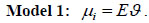
Model 1: The Poisson-Gamma model is sometimes used to model the relative risk of the number of child mortality in a district (state). The relative risk combines with the Poisson likelihood function for the death counts and Gamma prior distribution to yield a Gamma posterior distribution for the relative risk [36].
Let yi and Ei; i = 1;::: ; n, denote the observed and expected number of death cases in district (state) i. We assume the death count that yi ~ Poisson(Eϑ), where ϑ is the unknown relative risk and Poisson mean µi is modeled as
 |
(2) |
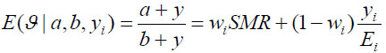
We assume that ϑ = Gamma(a,b) for i = 1::: 37 in our study n=37 districts (states) in Nigeria. By combining the likelihood and the prior distribution, the posterior mean or the relative is obtained as
 |
where
 ; represents a weighted average that indicates how much the posterior mean shrunk towards the individual expectation, Ei as explained in [37]. One advantage of the Poisson-gamma model is that it provides a simplified way to accommodate over-dispersion in the model. A drawback is that this Poisson-gamma model does not permit the inclusion of covariate(s) [36, 38].
Model 2: Clayton and Kaldor [16] first proposed a Poisson log normal model that combines the relative risk and a normally distributed random variable. The model includes area-specific random effects or spatially unstructured random effects, vi and ϑ is the overall level of the relative risk .
Using equation (1) above, µi = Eϑ, the log normal model for the relative risk becomes
 |
(3) |
where the linear link function η = log(ϑ) = X'β+vi
vi is the spatially unstructured random effects that were modeled as using the Gaussian prior distribution with a zero mean and the variance,
 i.e.vi ~ N(0,
) where
represents specific area variance. X is a vector of covariates (such as proportion of poor households, unimproved source of drinking water, unprotected toilet, children having diarrhoea, the proportion of mothers using solid fuels (coal, wood, agricultural residues cow dung etc) as cooking method . Thus, the relative risk provides a more flexible alternative to the independent Poisson model, as stated in [39].
i.e.vi ~ N(0,
) where
represents specific area variance. X is a vector of covariates (such as proportion of poor households, unimproved source of drinking water, unprotected toilet, children having diarrhoea, the proportion of mothers using solid fuels (coal, wood, agricultural residues cow dung etc) as cooking method . Thus, the relative risk provides a more flexible alternative to the independent Poisson model, as stated in [39].
Model 3: The conditional autoregressive (CAR) model has been widely used for the analysis of spatial data in different areas, such as demography, geography and epidemiology. This model was introduced by [40] as a spatial methodology to estimate disease risk, which assumed a spatial dependence with neighboring regions. The ui is the spatially structured (correlated) random effects were modeled using the conditional autoregressive prior distribution as suggested by [40].
Using equation (1) above, ui, the CAR model for the relative risk becomes
 |
(4) |
and the linear link function becomes η = log(ϑ) = X'β+ui
where ui
 where area i ~ j are adjacent (neighbours), and wij = 1 and zero if they are not. X is a vector of covariates (such as proportion of poor households, unimproved source of drinking water, the proportion of households using unprotected toilets, the number of children having diarrhoea, proportion of mothers using solid fuels (coal, wood, agricultural residues, cow dung etc) as cooking methods.
Model 4: Besag, York and Mollie (BYM) model was first introduced by [16] and later extended by [40]. BYM model is then split into two spatial random and heterogeneity components and it is formulated through the following equation. The death count assumes, yi ~ Poisson(ϑ) the log relative risk is modeled through equation (1) above, µi = Eϑ, and the BYM model for the relative risk becomes
 |
(5) |
and the linear link function becomes η = log(ϑ) = X'β + ui + vi
where vi and µi are unstructured and structured spatial random effects respectively. They are model as vi ~ N(0,
) and
where area i ~ j are adjacent (neighbours), wij = 1 and zero if they are not. X is a vector of covariates as stated above . The ϑ reflects the amount of extra Poisson variation in the data and
represents specific area variance as stated in [39]. The precision parameters τu2 and τv2 control the variability of u and v respectively. The parameter estimation was executed via the Bayesian Markov Chain Monte Carlo Convergence of the MCMC, which was reached at 15000 iteration after a burn-in period of 5,000 samples and the thinning was done at every 90th element of the chain. The statistical inference is based on full Bayesian framework and prior distributions were specified for the model parameters. The posterior estimates are used to explain the model results of the UH, CAR and the BYM model which are presented in Table 4.
The model performance was investigated via Deviance Information Criterion (DIC) which is due to Spiegelhalter et al. [41] given as
 |
(6) |
where D is the posterior mean of the deviance and
is the vector of model parameters. pD is the number of effective parameters in the model that penalizes its complexity. DIC takes into account both the model fit (summarized by D) and model complexity (captured by PD) when comparing models. Therefore, the model having the smaller value of DIC is the most preferred one as it achieves a more optimal combination of fit and parsimony.
The parameter estimation was done using Bayesian Markov Chain Monte Carlo via Gibbs Sampling. The convergence of the MCMC was achieved at 15,000 iterations after a burn-in period of 5,000 samples and thinning of every 90th element of the chain. The hyper-prior prior distributions assumed for the precision parameters, τu2, τv2 and τβ2 are Gamma distributions as τu2, ~ Г(0.05,0.005), τv2 ~ Г(0.05,0.005) and τβ2, ~ Г(0.05,0.005) respectively. The coefficients of the covariates of the regression model are assumed to be normally distributed given as, β ~ N(0,0.005). All model analyses were carried out in WinBUGS after [41] and data manipulation was done in R programming [42]
3. RESULTS AND INTERPRETATIONS
Table 2 presents the number of child deaths, total births, expected deaths, and relative frequency distribution. The study involved 31482 children born between 2008 and 2013, out of which 2886 children died before reaching the age of five. Zamfara recorded the highest child mortality and relative frequency of 229 (7.96) and the second highest occurred in Kano, 221(7.66). Both states are found in the north-western region of Nigeria. The lowest under-five mortality was recorded in Osun state of 21(0.73).
Table 3 presents the estimates of the parameters and goodness of fit for the hierarchical models discussed in the previous section. The non-spatial method (P-Gamma model) does not account for autocorrelation in the residuals, although they appear to perform reasonably well overall.
| Model | Name | D(θ) | pD | DIC |
|---|---|---|---|---|
| M1 | UH | 261.426 | 25.278 | 286.70 |
| M2 | PG | 256.885 | 31.217 | 288.10 |
| M3 | CAR | 262.233 | 24.163 | 286.40 |
| M4 | BYM | 260.267 | 25.043 | 285.31 |
| PLN 95 % CI |
UH 95 % CI |
CAR 95 % CI |
BYM 95 % CI |
|||||||||
|---|---|---|---|---|---|---|---|---|---|---|---|---|
| β0 | - | - | - | -0.136 | -0.209 | -0.065 | -0.137 | -0.182 | -0.093 | -0.138 | -0.196 | -0.080 |
| A | 10.31 | 6.23 | 15.97 | - | - | - | - | - | - | - | - | - |
| B | 11.20 | 6.68 | 17.35 | - | - | - | - | - | - | - | - | - |
| µ | 0.92 | 0.83 | 1.03 | - | - | - | - | - | - | - | - | - |
| σ2 | 0.09 | 0.05 | 0.14 | - | - | - | - | - | - | - | - | - |
| β1 | - | - | - | 0.052 | -0.460 | 0.614 | 0.130 | -0.452 | 0.698 | 0.173 | -0.372 | 0.730 |
| β2 | - | - | - | 0.350 | -0.149 | 0.875 | 0.362 | -0.100 | 0.857 | 0.353 | -0.190 | 0.851 |
| β3 | - | - | - | -0.095 | -0.650 | 0.427 | -0.247 | -0.762 | 0.291 | -0.226 | -0.771 | 0.333 |
| β4 | - | - | - | 1.653 | 0.773 | 2.491 | 2.088 | 1.088 | 3.165 | 2.003 | 1.101 | 3.006 |
| β5 | - | - | - | -0.306 | -1.066 | 0.520 | -0.491 | -1.383 | 0.350 | -0.516 | -1.591 | 0.430 |
| τu2 | - | - | - | 14.34 | 5.006 | 35.47 | 56.98 | 6.104 | 339 | |||
| σu | - | - | - | 0.291 | 0.168 | 0.447 | 0.221 | 0.054 | 0.405 | |||
| τu2 | - | - | - | 41.760 | 16.75 | 100.5 | - | - | - | 330.60 | 23.84 | 2101 |
| σv | - | - | - | 0.168 | 0.100 | 0.244 | - | - | - | 0.099 | 0.022 | 0.205 |
Although the CAR model and BYM model each provides important information about clustering of the childhood mortality relative risk pattern, one would recommend that the BYM is the best fitted model for Nigerian child mortality data, since it yielded the lowest value of the DIC = 285:310 and with a lower pD= 25.04. The CAR model had DIC= 286.40 and pD=(24.16) as the goodness of measure and it competes closely with the BYM model. However, the BYM model is the most preferred one due to its robustness and at the same time one can evaluate the proportional of variation that can be attributed to spatial dependence (clustering) and the variation due to random heterogeneity effect structure of the mortality prevalence.
Table 4 presents the posterior statistics of the fitted hierarchical models. It can be observed that the posterior mean of P-G model is 0.923: 95% CI (0.826, 1.030), which is approximately the same as the mean of the SMR of 0.920 and standard deviation, 0.306. The overall population parameters, a = 10:310; (6:232; 15:970) and b = 11:200(6:680; 17:350) from the Poisson Gamma model. The Poisson -log normal (PLN) model yielded a precision variance of, τv2= 41.76 with a standard deviation of 0.168. This indicates that the relative risk of child mortality at any given state is similar (less heterogeneous) to that of its neighbours. The CAR model's precision variance, τu2 =14:34; (5,006 to 35.47) and standard deviation of 0.291, which indicates that the geographic patterns of under five mortality exhibits more of clustering across the selected administrative units (states)in Nigeria. The precision variance parameter of the BYM model has CAR precision variance,
 = 56.98; 95% CI (6.104, 339.0) and σu = 0.291. In other words, the small value of standard deviation,σu = 0.291 of spatial structured random effects, which means that the neighbours are not independent. The spatial heterogeneity component of variation in the BYM model has precision variance,
 = 330.60, 95%CI (23.84, 2101) and σv = 0.099. From the BYM model analysis, one can deduce the proportion of the variation that is due to clustering as
 = 69.06% and the proportion of variability attributed to the heterogeneity random effect is 1 -α = 30.93%.
The results revealed further that the geographic patterns of the under-five mortality prevalence in Nigeria exhibit more clustering than the spatial heterogeneity variation, as evidenced from the estimates. The geographic pattern of variation of the under-five mortality can be attributed to clustering from the exposure to local environmental factors, underlying ecological indices or severity of poverty index at the community level.
| RR < 0.050 | RR : 0.050-0.990 | RR > 1 | |||||||||
|---|---|---|---|---|---|---|---|---|---|---|---|
| Significant low | Not significant | Significant high | |||||||||
| Osun | 0.572 | (0.572, | 0.714) | Akwa Ibom | 0.807 | (0.640, | 1.006) | Sokoto | 1.316 | (1.133, | 1.515) |
| Edo | 0.591 | (0.591, | 0.736) | Enugu | 0.813 | (0.646, | 1.013) | Ebonyi | 1.326 | (1.101, | 1.586) |
| Fct-abuja | 0.625 | (0.625, | 0.806) | Imo | 0.842 | (0.646, | 1.076) | Bauchi | 1.352 | (1.178, | 1.548) |
| Kwara | 0.635 | (0.635, | 0.791) | Rivers | 0.846 | (0.681, | 1.033) | Kebbi | 1.362 | (1.160, | 1.594) |
| Ekiti | 0.645 | (0.645, | 0.815) | Plateau | 0.939 | (0.752, | 1.142) | Jigawa | 1.439 | (1.252, | 1.645) |
| Borno | 0.680 | (0.680, | 0.860) | Adamawa | 1.018 | (0.843, | 1.218) | Zamfara | 1.680 | (1.479, | 1.910} |
| Kogi | 0.680 | (0.680, | 0.820) | Benue | 1.063 | (0.876, | 1.264) | ||||
| Oyo | 0.699 | (0.699, | 0.876) | Katsina | 1.083 | (0.926, | 1.249) | ||||
| Kaduna | 0.708 | (0.708, | 0.850) | Kano | 1.088 | (0.951, | 1.231) | ||||
| Ogun | 0.708 | (0.708, | 0.885) | Yobe | 1.105 | (0.926, | 1.300) | ||||
| Lagos | 0.711 | (0.711, | 0.881) | Taraba | 1.125 | (0.964, | 1.294) | ||||
| Delta | 0.726 | (0.726, | 0.881) | Gombe | 1.139 | (0.969, | 1.327) | ||||
| Niger | 0.736 | (0.736, | 0.875) | ||||||||
| Bayelsa | 0.762 | (0.762, | 0.960) | ||||||||
| Ondo | 0.773 | (0.773, | 0.936) | ||||||||
| Anambra | 0.781 | (0.781, | 0.964 | ||||||||
| Abia | 0.793 | (0.793, | 0.964) | ||||||||
| Nasarawa | 0.801 | (0.801 | 0.984) | ||||||||
| Cross river | 0.801 | (0.801 | 0.994) | ||||||||
| RR < 0.050 | RR : 0.050-0.990 | RR > 1 | |||||||||
|---|---|---|---|---|---|---|---|---|---|---|---|
| Significant low | Not significant | Significant high | |||||||||
| Osun | 0.566 | [0.420, | 0.726] | Anambra | 0.801 | [0.637, | 1.008] | Sokoto | 1.310 | [1.127, | 1.511] |
| Edo | 0.580 | [0.443, | 0.733] | Akwa Ibom | 0.802 | [0.628, | 1.001] | Ebonyi | 1.321 | [1.092, | 1.590] |
| Fct-Abuja | 0.633 | [0.474, | 0.818] | Enugu | 0.817 | [0.641, | 1.015] | Bauchi | 1.358 | [1.181, | 1.547] |
| Ekiti | 0.659 | [0.511, | 0.840] | Rivers | 0.826 | [0.648, | 1.024] | Kebbi | 1.362 | [1.166, | 1.576] |
| Kwara | 0.662 | [0.525, | 0.828] | Imo | 0.832 | [0.636, | 1.068] | Jigawa | 1.443 | [1.257, | 1.640] |
| Kogi | 0.669 | [0.526, | 0.827] | Nasarawa | 0.835 | [0.666, | 1.042] | Zamfara | 1.696 | [1.491, | 1.922] |
| Borno | 0.672 | [0.497, | 0.859] | Plateau | 0.926 | [0.738, | 1.135] | ||||
| Kaduna | 0.697 | [0.556, | 0.848] | Adamawa | 1.030 | [0.854, | 1.224] | ||||
| Oyo | 0.703 | [0.542, | 0.880] | Benue | 1.042 | [0.839, | 1.252] | ||||
| Lagos | 0.709 | [0.550, | 0.885] | Katsina | 1.067 | [0.910, | 1.234] | ||||
| Niger | 0.718 | [0.578, | 0.866] | Kano | 1.091 | [0.960, | 1.231] | ||||
| Delta | 0.724 | [0.576, | 0.891] | Yobe | 1.102 | [0.918, | 1.302] | ||||
| Ogun | 0.724 | [0.557, | 0.921] | Taraba | 1.112 | [0.948, | 1.284] | ||||
| Bayelsa | 0.762 | [0.601, | 0.946] | Gombe | 1.151 | [0.982, | 1.339] | ||||
| Ondo | 0.785 | [0.627, | 0.969] | ||||||||
| Abia | 0.786 | [0.626, | 0.968] | ||||||||
| Cross river | 0.787 | [0.617, | 0.980] | ||||||||
Furthermore, the risk factors are presented along with posterior statistics in Table 4. The results revealed that the estimated intercept, relative risk effect of the models are: PLN β 0 = -0.137; 95%CI (-0.209, -0.075), CAR: β 0 = -0.137, (-0.182, -0.092), and BYM model: β 0 = -0:138, 95% CI (-0.200, -0.080). These risk effects are significantly different from zero and negative. These models (CAR and BYM) consolidate the result of the UH model that indicates the overall child mortality risk. A negative coefficient intercept indicates a decreasing relative risk of childhood mortality by keeping the (fixed covariates) determinant factors of under-five mortality constant. The household poverty variables are significant and positive for all the models (UH, CAR and the BYM) with these parameter estimates UH: 1.653, 95% CI (0.773, 2.491), CAR: 2.088 95%CI (1.088, 3.165), BYM: 2.003, 95%CI (1.101, 3.006). The results showed that the household poverty level would increase the relative mortality risks among the children who belong to the most economically deprived households. Other covariates in the model were not significant for the childhood mortality. However, the children who suffered from diarrhoea and who used unhygienic toilets/ sanitation had a higher tendency to die before reaching the age of five (i.e. positive association with the under- five child mortality), although they were not significant in this case. Children from mothers who used solid fuels (such as charcoal, coal, wood or agricultural residues) for cooking and drank from unprotected water are negatively insignificant.
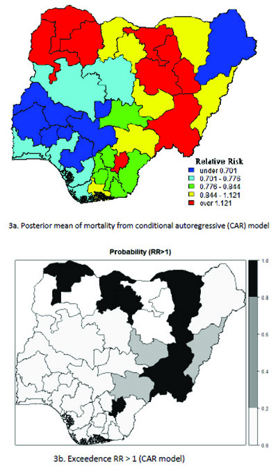
Table 5 presents the results of the conditional autoregressive (CAR) model with the classification of the states according to the relative risk (RR) value of childhood mortality prevalence and significance probability (RR > 1) for UH model. The geographical variation in the relative risk values range from 0.438 to 1.910. The relative risk above 1(RR >1.000) indicates that the under-five mortality prevalence are higher in those states. The lowest estimated risk value occurred in Osun state: 0.0.572 (0.438, 0.714) and highest risk was recorded in Zamfara:1.680 (1.479 to 1.910). In the risk map displayed in Fig. (3), the geographical variation ranges from 0.420 to 1.922. Out of the 37 districts, the BYM model classified six (6) states as having a high relative risk of under- five mortality (RR >1.000). The relative risk value for the mortality ranges from the lowest Osun state: 0.566(0.42, 0.73) to the highest risk in Zamfara: 1.696 (1.491, 1.992). These showed that six (6) states had a relative risk significantly above 1 Table 6.
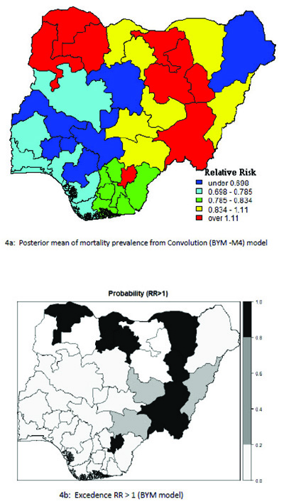
The probability risk map displayed in Fig. (4) represents smooth map of mortality for the BYM model and the states with relative risk value greater than 1. This is considered as an indication of a lower prevalence of under-five child mortality detected in the south western states and a high prevalence of mortality was found in the northern regions of the country.
4. DISCUSSION
In this study, a Bayesian hierarchical model was employed to assess the child mortality risk and potential risk factors such as socio-cultural and environmental factors for under-five mortality in Nigeria. The strength of the approach is the ability to incorporate high over-dispersion, spatial structure and covariates into the models.
The result shows that household poverty is significantly associated with under-five mortality in Nigeria. In other words, an economically deprived household has higher likelihood of childhood mortality. This finding corroborates what has been established in previous studies. These have shown that people’s living conditions and household poverty influences virtually the totality of the demographic structure and health indices, including life facilities, and even human capital development as reported in [43-45]. A similar study conducted in Nigeria by [46] using data from 1990-2008 found that household wealth had a strong association with not only under-five mortality, but also with the other house members life expectancy, maternal mortality and morbidity, fertility, contraceptive use and the use of healthcare .
The results also reveal that poor toilet sanitary conditions and unimproved sources of drinking water are positively associated with childhood mortality, although these factors are not significant. In contrasts, a previous study conducted by [47], who introduced similar biophysical/geographical variables into their model of child malnutrition, found that these factors are significantly correlated with child malnutrition: drought prevalence, the percentage of households with piped water, and diarrhoea disease prevalence.
Furthermore, the probability risk maps reveal that there are clusters of high mortality risk concentrated in the northern regions of Nigeria. These outcomes can be attributed to the complexities such as cultural factors, socio-demographics, severity of household poverty, climate and drought, lack of access to portable water, open toilets, house structure and individual household environments. The findings are in complete agreement with the study conducted in Mozambique by [48]
The results in Table 4 showed further that there are no significant relationships between drinking water sources and under-five mortality. However, the findings from other studies conducted by [49, 50] have demonstrated the positive impact of access to clean water as significant for under-five mortality, while the problem of unsafe drinking water, inadequate water for food and personal hygiene, and insufficient access to sanitation have been identified as partly responsible for about 88% of child deaths from infectious diseases, and mostly repeated diarrhoea in children globally, as reported in [51, 52]. Other studies have established that a high proportion of children deaths in low-middle income countries can be attributed to diseases resulting from poor housing conditions, unsafe water supply, inadequate sanitary facilities, unhygienic behaviour and household air pollution from solid cooking fuels - wood, charcoal, and agricultural residues [53, 54].
The probability risk maps presented in this study highlight geographic disparities and relative high mortality risk among young children in Nigeria, mostly found in the northern parts of the country. The results corroborate the findings from previous studies conducted in Nigeria by [55], who used a scan statistic method and by [56], who used an exploratory spatial analysis. The persistent high risk of child mortality found in the northern regions can be related to environmental factors, neighbourhood structure, education and economic deprivation. Our findings are in tandem with a study conducted in other West African countries such as, Ghana, where researchers detected non-random patterns or clusters of high child mortality at village level with a large concentration of polygamous population or nuclear family settings as reported by [57].
The statistical issues relating to disease mapping and modelling of aggregated data of rare disease have been extensively discussed in [36], while [58] had earlier investigated the small area clustering of under-five mortality in Ethiopia. Previous studies have explored mixture models, for example, the study conducted by [59], where researchers combined a convolution model and Poisson-Gamma model to account for both over-dispersion and spatial correlation in the modeling of kidney and prostate cancer data. A wide range of distributions have been derived with Poisson distribution because of its positive parameter value, see ([60, 61] for more discussion).
This present study consolidates the existing literature such as [12, 13, 62], reported that the health impacts of climate change, geography and the local environment where people live had significant association with their health outcomes. Furthermore, health inequalities are partly a reflection of social inequalities, which are more widely defined among sub-populations even in developed countries, according to the studies by [17, 20]. A compressive assessment of the health impacts of climate change and geography scale was discussed in [62-64]. In their study, they emphasized that complex processes operating at various geographical scales linking global health with the local and individual characteristics made a significant contribution to health determinants. The findings from the present study can assist healthcare givers and government agencies to address the geographic disparities in the mortality prevalence and design needed interventions.
CONCLUSION
The proposed models and the results reveal that there are apparently geographical inequalities of child mortality prevalence across the states in Nigeria. The maps highlight clusters of high under-five mortality prevalence in the northern states and in an isolated case of Ebonyi (in the south eastern region) during the study period. Therefore, these states (regions) are in need of urgent attention and interventions. However, a relatively low prevalence of childhood mortality was observed in the south-western parts of Nigeria. The findings can guide in evidence-based allocations of scarce health resources in the sub-region with the aim of improving the chance of child survival. Our methodology was motivated by two specifications, the first of which assessed spatial dependence by borrowing strength from neighbouring states (districts) to identity clusters of child mortality in Nigeria. Secondly, the model investigated the impact of spatial heterogeneity, as a way of evaluating geographical disparities in child mortality prevalence across the regions in Nigeria.
LIST OF ABBREVIATIONS
| NDHS | = Nigeria Demographic and Health Survey |
| SMR | = Standardized Mortality Ratio |
| MCMC | = Markov chain Monte Carlos |
| MDGs | = Millennium Development Goals |
| DRC | = Democratic Republic of Congo |
| DSS | = Demographic Surveillance Sites |
| MAUP | = Modifiable Areal Unit Problems |
| USAID | = United States Agency for International Development |
| FCT | = Federal Capital Territory |
AUTHORS' CONTRIBUTIONS
RAA, TZ and SR conceptualized the idea for the study. RAA acquired the data, performed the analysis, and drafted the manuscript. TZ suggested the research proposal and advised on the statistical methodology. Both TZ and SR read the first draft and made relevant comments. RAA implemented the suggestions and comments on manuscript. All authors read the final manuscript preparation and approved the submission.
ETHICS APPROVAL AND CONSENT TO PARTICIPATE
Not applicable.
HUMAN AND ANIMAL RIGHTS
No animals/humans were used for studies that are the basis of this study.
CONSENT FOR PUBLICATION
Not applicable.
AVAILABILITY OF DATA AND MATERIALS
The data used for this study can be obtained by requesting the ORC macro and DHS.
FUNDING
No funding was awarded to this article.
CONFLICT OF INTEREST
The authors declare no conflict of interest, financial or otherwise.
ACKNOWLEDGEMENTS
The authors would like to acknowledge the permission granted by DHS, Calverton Macro, USA and the National Bureau of Statistics, Abuja-Nigeria to use the DHS data. The first author also appreciates the study leave/fellowship enjoyed from the Federal University of Technology, Minna Niger state, Nigeria to undergo his postgraduate research study in South Africa.