All published articles of this journal are available on ScienceDirect.

A Review of Outlier Detection Methods: From Visual Inspection to Advanced Algorithms

Abstract
Introduction/Objective
Outlier detection is a fundamental component of data preprocessing that aims to identify anomalies that may arise from measurement errors, data entry errors, system failures, fraudulent activities, or rare but meaningful events. The aim of this study is to provide a comprehensive overview of outlier detection methods, ranging from traditional statistical and visualization techniques to advanced machine learning and deep learning approaches.
Methods
This review presents a structured taxonomy of outlier detection methodologies, progressing from fundamental visual methods (box plots, scatter plots, histograms) through statistical methods (parametric: Z-score, regression-based; non-parametric: kernel density estimation), distance-based methods (local neighborhood, kNN-distance), density-based techniques (LOF, COF, INFLO, MDEF), and clustering-based approaches (k-means, hierarchical, DBSCAN). We extend coverage to advanced algorithms including Isolation Forest, Feature Bagging, and deep learning-based autoencoders, with a simulated medical case study and reproducible R code.
Results
No universally superior method exists; performance is highly context-dependent. Advanced algorithms demonstrate superior scalability and effectiveness in high-dimensional and complex data environments, albeit with increased computational requirements and reduced interpretability. In our simulated medical case study, Isolation Forest achieved the highest sensitivity (0.97) for detecting injected anomalies.
Discussion
This study shows that no single outlier detection technique is suitable for all scenarios. The selection of an appropriate method should be done considering the data structure, dimensions, and specific requirements for reliable anomaly detection.
Conclusion
Methodological selection requires careful consideration of data properties, computational constraints, and analytical goals. We provide a practical, reproducible framework integrating domain expertise with modern algorithmic approaches.
1. INTRODUCTION
Ensuring data integrity and quality is still crucial in today's data-driven decision-making environment. The presence of outliers-observations that significantly deviate from the majority pattern-poses serious analytical challenges alongside other data quality issues [1]. These unusual occurrences could be the result of inaccurate measurements or errors in data processing, or they could be actual new phenomena like uncommon illnesses or security lapses. Therefore, correctly identifying outliers is a crucial analytical step because their presence can significantly distort statistical estimates, jeopardize the integrity of the model, and eventually result in incorrect conclusions [2, 3].
Outlier detection, also known as anomaly detection, is a methodological field that has experienced significant development, producing a wide range of methods from simple statistical tests to complex machine learning algorithms [4]. Although the operational definition of “expected” differs significantly across methodological paradigms, the basic goal remains the identification of data points that do not conform to expected patterns. While some methods rely on specific statistical distributions, others use geometric distance measures or local density measures to conceptualize outliers [5].
Unlike prior surveys, this tutorial paper (i) provides a complete taxonomic progression from basic to advanced methods, (ii) includes a transparent literature search methodology, (iii) introduces modern algorithms (Isolation Forest, Feature Bagging, Autoencoders) often omitted in educational reviews, and (iv) offers a reproducible medical case study with R code enabling readers to implement and visualize outlier detection methods immediately [6-8]
2. METHODS
2.1. Literature Search Methodology (Transparency Statement)
This article is conceived as a narrative tutorial review rather than a systematic review or meta-analysis. Consistent with narrative review conventions, we conducted a purposeful, iterative literature search rather than an exhaustive systematic search (Byrne, 2016). The search strategy is summarized below:
| Parameter | Specification |
|---|---|
| Databases consulted | PubMed, Scopus, Google Scholar |
| Time frame | January 2000 – December 2025 |
| Search keywords |
(“outlier detection” OR “anomaly detection”) AND (“statistical” OR “distance-based” OR “density-based” OR “clustering” OR “isolation forest” OR “autoencoder” OR “ensemble”) |
| Search approach |
Purposeful, iterative, snowballing (reference lists of key papers) |
| Inclusion criteria |
Peer-reviewed articles, conference proceedings, methodological tutorials, and influential textbooks in English |
| Exclusion criteria |
Non-English articles, unpublished preprints, opinion pieces without methodological content |
| Selection basis |
Author judgment based on educational value, methodological representativeness, and clinical relevance |
This search yielded approximately 400 initial records. After removing duplicates and screening for educational relevance, approximately 15 core references were selected for inclusion [6, 9-22]. The selection process prioritized methodological diversity and pedagogical clarity over exhaustive enumeration.
3. A TAXONOMY OF OUTLIER DETECTION METHODS
The outlier detection methodological ecosystem has considerable diversity, providing multi-layered approaches for identifying abnormal data observations. These methods, ranging from fully automated computer algorithms to human-centric representations, can be systematically grouped based on underlying theoretical principles. A basic organizational structure considers progression from simple to sophisticated approaches. Initial methods provide essential baseline data assessment by utilizing human cognitive capacities through graphical representations. More elaborate model-driven approaches are required as data dimensionality and volume increase [9].
These advanced methodologies operate under divergent core assumptions regarding the constitution of outliers, whether defined as deviations from statistical models, geometric isolation from neighboring points, occupancy of low-density regions, or failure to associate with natural data clusters. Comprehending this taxonomic structure extends beyond academic interest, serving as a practical decision framework for analysts to select appropriate tools that ensure reliable and meaningful outlier identification [6, 23].
3.1. Visual Methods: The First Line of Defense
Visual inspection is an essential first step in analytical workflows before implementing complicated computational methods. These methods leverage human pattern recognition capabilities to quickly understand global data structures and identify noticeable irregularities that might evade automated detection. Their key advantages are rapid interpretability and operational simplicity, allowing domain experts to identify data anomalies or novel patterns without requiring sophisticated statistical training. However, data complexity and human perceptual limitations naturally constrain visual method effectiveness. These methods demonstrate maximal utility in univariate or bivariate analyses but become progressively less effective in high-dimensional settings [24].
3.1.1. Box Plot
The box plot, also called a box-and-whisker plot, is a standardized visualization technique for displaying the distribution of data using a five-number summary: minimum, first quartile (Q1), median, third quartile (Q3), and maximum. The Interquartile Range (IQR), containing the central 50% of observations, defines the “box” dimension, while “whiskers” typically extend to extreme values within 1.5 × IQR from the quartiles. Observations exceeding these boundaries receive individual plotting and constitute potential outliers [25].
This methodology proves particularly effective for identifying distributional skewness and facilitating cross-categorical distribution comparisons. Its non-parametric nature ensures robustness, operating without presupposing underlying statistical distributions. In clinical contexts, box plots of patient laboratory values (e.g., cholesterol levels) can immediately flag individuals with extreme values relative to reference populations, prompting further medical evaluation.
Statistical Formulation
The outlier detection threshold follows:
Lower Bound=Q1−1.5×IQR
Upper Bound=Q3+1.5×IQR
where IQR=Q3−Q1
As illustrated in Fig. (1), the box plot provides a visual summary of the glucose level distribution and enables identification of observations located beyond the Interquartile Range (IQR), which may represent potential outliers.
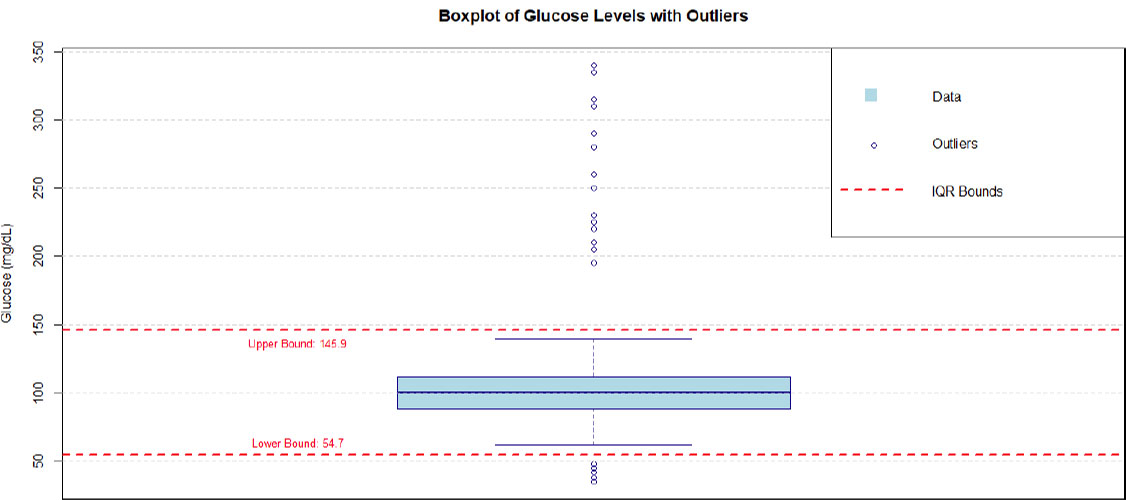
Box plot of glucose levels.
3.1.2. Scatter Plot
In bivariate data, scatter plots are essential visual tools for identifying outliers, allowing observation of patterns in relationships between two continuous variables. Cartesian coordinates of each plot correspond to each observation. In this framework, outliers appear as points that deviate from the main pattern or concentration created by most observations. Extreme values in a single dimension, unusual combinations of variables, or notable departures from observable correlation trends (such as linear relationships) exemplify these anomalies.
In epidemiological research, scatter plots analyzing Body Mass Index (BMI) against blood glucose levels may reveal patients exhibiting normal BMI with exceptional glucose measurement combinations warranting clinical investigation. While scatter plots effectively reveal contextual outliers and non-linear patterns, their application remains restricted to two-dimensional representation [26].
Figure 2 demonstrates the relationship between BMI and fasting glucose levels, in which observations deviating from the main distribution can be visually identified as potential contextual outliers.
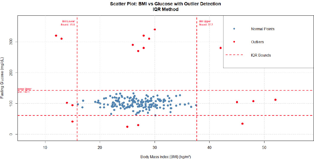
Scatter plot of BMI vs. fasting glucose.
3.1.3. Histogram
By dividing the data range into successive, non-overlapping intervals (bins), histograms provide graphical distribution approximations for numerical variables. Bar height correlates with observation frequency (or density) within each bin. Outliers appear as solitary bars distant from the main distribution mass, representing infrequent values [25].
Bin width selection remains crucial for method success; an excessive width may conceal outliers by grouping normal data, while an insufficient width produces spiky, fragmented distributions that complicate interpretation. Histograms are primarily used for univariate analysis but also facilitate rapid normality testing, skewness evaluation, and multimodality identification.
Figure 3 presents the histogram distribution of glucose levels, illustrating the overall data pattern and highlighting extreme observations away from the central frequency distribution.
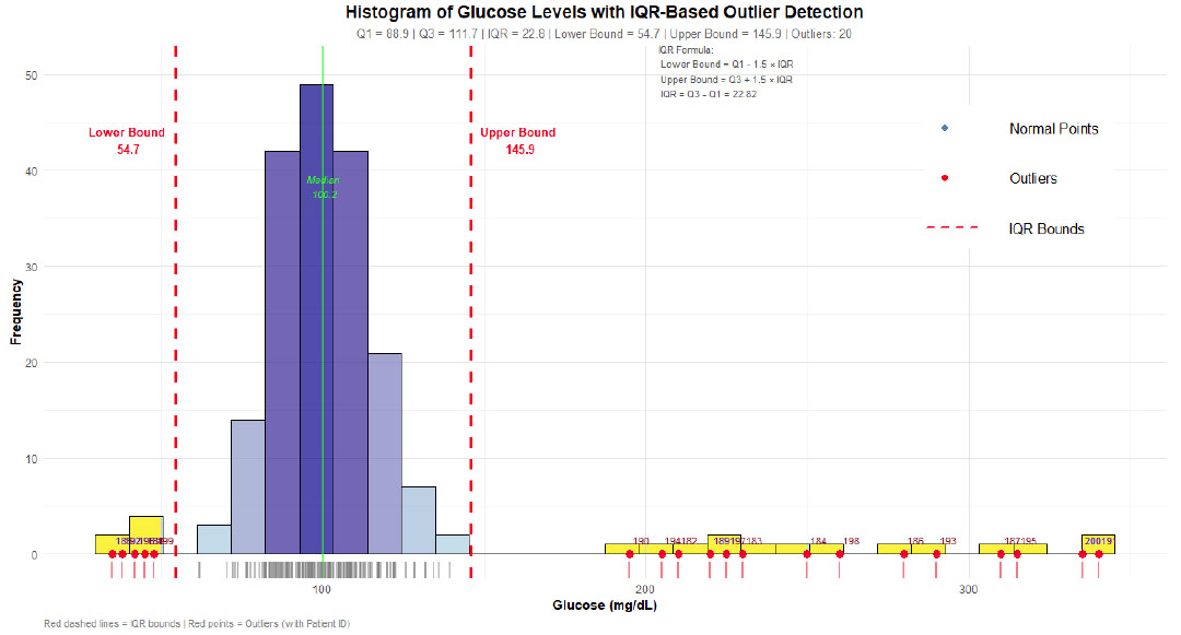
Histogram of glucose levels.
3.2. Statistical Methods
Statistical techniques constitute the traditional foundation of outlier detection, employing well-established statistical theory to characterize and detect anomalies. These methods operate by first fitting probabilistic models to data, then flagging observations showing low generation probability under the presumptive model. The fundamental strength of statistical methods is their mathematical rigor, enabling the construction of confidence intervals around “normal” data patterns and probabilistic interpretation. However, this advantage also represents their main drawback, as most parametric statistical techniques require strong assumptions about underlying data distributions (e.g., normality). Methodological performance degrades when these assumptions prove incorrect, potentially leading to the omission of genuine outliers or excessive false positives. Furthermore, these techniques often struggle with the “curse of dimensionality,” where conceptualizing tail behavior in multivariate distributions becomes increasingly complex [27].
3.2.1. Parametric Methods
3.2.1.1. Gaussian Distribution
Parametric approaches presuppose that data adhere to specific, known probability distributions, with the Gaussian distribution being the most prevalent foundational assumption. Under this paradigm, data characterization occurs through mean (μ) and standard deviation (σ) parameters. Outlier identification subsequently focuses on observations demonstrating extreme deviation from the mean, typically quantified through Z-score standardization [28].
This methodology offers computational efficiency and straightforward implementation across statistical platforms (SPSS, R, STATA). Clinical laboratory medicine frequently employs this approach, establishing reference ranges as mean ± 2 standard deviations for biological biomarkers.
Statistical Formulation:

where observations with |Z| > 3 (or sometimes 2.5) are considered potential outliers, corresponding to approximately 0.3% of data under perfect normality.
3.2.1.2. Regression-based
Regression-based outlier detection represents a powerful parametric method for identifying anomalies in variable-relationship contexts. The process begins with estimating a regression model (linear or nonlinear), establishing predictive relationships between independent and dependent variables. Subsequently, residual analysis-differences between observed and model-predicted values-becomes the focus of outlier detection. Observations with large residuals (Y-direction outliers) indicate model violations, while high-leverage points (X-direction extremes) may be influential outliers that can substantially distort parameter estimations [29].
Statistical Formulation:
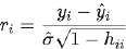
For a regression model yi=β0+β1xi+ϵi, standardized residuals are calculated as:
where hii represents the leverage of the i-th observation.
3.2.2. Non-Parametric Methods
3.2.2.1. Kernel Density Estimation
Kernel Density Estimation (KDE) is a sophisticated non-parametric method for estimating probability density functions without assuming distributional forms. Rather than using discrete bins as in histograms, KDE places smooth kernel functions (e.g., Gaussian densities) at each observation and integrates them to obtain continuous density estimates. Observations falling into regions with the lowest estimated probability density are identified as outliers [30].
The main benefit of KDE over histograms is that it eliminates arbitrary dependencies on bin origin and width, resulting in distributional estimates that are smoother and more reliable. Density smoothness is controlled by the crucial bandwidth parameter; excessive bandwidth results in over-smoothing that could mask real outliers, while insufficient bandwidth produces overfitting and artificial density fluctuations. Applying KDE to daily ER admissions in hospital administration could reveal days with unusual patient volumes that deviate from typical trends. When typical parametric models show poor fit, KDE provides flexible, powerful distribution modeling for outlier discovery, even though it requires more computing power than basic histograms.
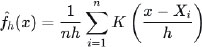
where K represents the kernel function and h the bandwidth parameter.
3.2.3. Distance-based Methods
Distance-based methodologies emerged to address limitations of statistical distributional assumptions, introducing geometric, non-parametric perspectives on outlier detection. The foundational intuition remains elegantly simple: conventional data points inhabit dense neighborhoods, whereas outliers exhibit isolation by being substantially distant from their neighbors. These techniques operate without prerequisite model fitting or distributional assumptions, relying exclusively on proximity measures, typically Euclidean or Manhattan distance in multidimensional spaces. This confers substantial versatility for application across diverse datasets with unknown or complex underlying distributions. Their primary advantage involves conceptual transparency and interpretative accessibility. However, methodological performance remains heavily influenced by distance metric selection and critical parameters, including neighbor count (k) or distance thresholds (λ). A significant challenge, the “curse of dimensionality,” manifests in high-dimensional spaces where interpoint distances tend toward uniformity, complicating discrimination between normal and outlier observations based solely on distance metrics [31].
3.2.3.1. Local Neighborhood (DB (k, λ)-Outlier)
The DB (k, λ)-Outlier method, introduced by Knorr and Ng, represents one of the earliest and most intuitive distance-based outlier formalizations. A point p attains outlier status if fewer than k neighboring points reside within distance λ. This essentially establishes a “local neighborhood” of radius λ around each point; insufficient neighborhood density indicates anomalous behavior. This methodology demonstrates strength through conceptual simplicity and its capacity to handle multi-cluster datasets, defining outliers relative to the immediate vicinity rather than the global data distribution. The principal drawback lies in the critical yet challenging selection of the parameter λ. Overly conservative λ values may misclassify normal points in sparse regions as outliers, while excessively liberal values may preclude outlier detection entirely. This challenge intensifies in high-dimensional data environments, where defining meaningful spherical neighborhoods becomes problematic due to inherent data sparsity. Despite parametric sensitivity, the DB-outlier concept established foundational principles for subsequent neighbor-based methodologies.
3.2.3.2. kNN-distance Methods
kNN-distance approaches avoid the problems of fixed-radius λ selection by refining the local neighborhood concept through relative, rank-based outlier definitions. These methods use the distance between a point and its k-th Neighbor (Dk) as an outlier-ness metric instead of preset distances. Dk values are then used to rank the points, with the top n most distant observations being classified as outliers [32].
Because “neighborhood” dimensions automatically change to local data density, this methodology exhibits greater adaptability than fixed-radius systems. While single points indicate large distances, k-th neighborhoods remain small within dense clusters. Applying kNN distance to patient vital signs in clinical diagnostics could successfully identify patients with distinct physiological profiles by ranking individuals based on how different they are from their k most similar counterparts. This approach is widely used in specialist packages and data mining tools (e.g., dbscan in R). Compared to fixed-radius paradigms, the method typically shows improved resilience and practicality for real-world applications, even though parameter k selection is still required.
3.2.4. Density-based Methods
Density-based approaches introduce complex, relatively outlier-ness conceptualizations and mark a significant advancement over distance-based approaches. Density-based techniques compare local point density with adjacent point densities, whereas distance-based approaches take absolute distances to neighbors into account. The basic realization is that outliers are not just far-off points but also points that occupy regions with significantly lower density than their surroundings. This makes it possible to successfully identify outliers that reside in sparse regions adjacent to dense clusters, where basic distance-based techniques often fall short [33].
Points on the periphery of a cluster, for example, may exhibit significantly larger nearest-neighbor distances while retaining local densities similar to those of their clusters, making them non-strong outliers. In heterogeneous datasets with clusters that have different densities and shapes, density-based approaches perform exceptionally well. Nevertheless, this intricacy comes at a computational cost: these methods exhibit higher intensity, necessitating local density calculations and kNN searches for every point, as well as complex parameters that require meticulous optimization.
3.2.4.1. LOF (Local Outlier Factor)
The Local Outlier Factor (LOF) algorithm represents a pioneering, highly influential density-based methodology. Rather than examining distances to isolation, LOF computes scores representing point-specific outlier degrees. For a given point p, LOF constitutes the ratio between the average local density of its k-nearest neighbors and its own local density. When p demonstrates density comparable to its neighbors, LOF approximates 1, indicating normal inlier status. When p occupies sparser regions than its neighbors, LOF substantially exceeds 1, designating outlier status [33].
This relative measurement enables LOF to effectively handle scenarios involving clusters with divergent densities. Points within sparse clusters may exhibit large absolute neighbor distances yet maintain low LOF due to density similarity with their neighbors. Conversely, points within dense clusters demonstrate substantially lower density than their immediate neighbors, which receive high LOF scores. This makes LOF particularly powerful for complex, real-world data, though careful selection of the MinPts (k) parameter-which defines neighborhood size-remains essential.
3.2.4.2. COF (Connectivity-based Outlier Factor)
The Connectivity-based Outlier Factor (COF) emerged to address specific LOF limitations. LOF performance may deteriorate when outliers occupy low-density regions connected to clusters, such as inter-cluster “bridges” or cluster “tails.” Under these conditions, the local density of outliers may approximate the neighbor densities, producing LOF scores near 1 and leading to outlier omission [34].
COF addresses this through “connectivity” considerations between points and neighbors. The methodology introduces the “chaining distance” or “SBN-path” (Set-Based Nearest path) concepts, which measure the minimal total distance connecting points to their neighbors via nearest-neighbor sequences. COF scores derive from average chaining distances. Well-connected points (inliers) exhibit minimal average chaining distances, while outliers demonstrate “isolation” through connectivity measures, requiring elongated connection paths to neighborhoods and consequently producing elevated COF scores. This enhances sensitivity for outlier detection in challenging, connected low-density regions [35].
3.2.4.3. INFLO and MDEF
INFLO (Influenced Outlierness) and MDEF (Multi-granularity Deviation Factor) constitute advanced density-based methods designed for complex scenarios. INFLO enhances LOF through incorporation of both k-nearest neighbors (kNN) and “reverse nearest neighbors” (RNN). The RNN set for point p contains all points having p within their kNN sets. RNN inclusion provides symmetric, robust density estimation, particularly valuable in regions with significant density variation, preventing incorrect outlierness estimation [36].
MDEF operates on divergent principles, examining data across multiple “granularities” or scales (defined by radius values r). For each point, MDEF calculates the local neighborhood density deviation from the average density of neighbors across scales. Points demonstrating significant density deviation at any scale receive outlier designation. This multi-scale approach enables MDEF sensitivity to outliers that are apparent only through specific analytical “lenses” or resolutions, establishing a powerful capability for anomaly detection in complex, multi-density datasets.
3.2.5. Clustering-based Methods
By leveraging the intrinsic clustering algorithm's ability to group similar data points, clustering-based procedures provide distinctive, often effective detection approaches. According to this paradigm, observations that show a weak correlation with any cluster are considered outliers. These could be unassigned points, points that are assigned to sparse or minimal clusters, or points that are located on the periphery of distant clusters. This method demonstrates strong intuitiveness, which is consistent with human cognitive processes that recognize abnormalities as background “noise” or non-conforming items. Outlier detection, such as clustering by-products, is a major benefit and may save processing resources when clustering is the main analytical goal. However, a basic drawback is total reliance on the suitability and quality of the clustering technique. When clustering methods fail to identify natural groups in the data, outlier identification similarly fails. These techniques generally lack dedicated outlier-detection optimization, potentially demonstrating reduced sensitivity compared to specialized density-based or distance-based methodologies [37].
3.2.5.1. Partitioning Methods (k-means)
Datasets are divided into predefined k non-overlapping clusters using partitioning clustering techniques, such as k-means. Outlier identification uses a variety of methods after cluster formation. The most popular approach assigns cluster centroids and computes the distances between points. Outlier classification is used for observations that show distances significantly greater than usual within-cluster lengths. Other methods treat minimum clusters (those with few points) as groupings of outliers. Although K-means offers scalability and computational efficiency for large datasets, it has a few disadvantages when it comes to outlier detection. The methodology assumes that clusters are spherical and of similar sizes, which is often broken in real-world applications. Additionally, during clustering operations, outliers can significantly alter centroid positions, leading to poor cluster formation and, in turn, insufficient outlier identification. For preliminary assessments, operational simplicity and speed of execution remain appealing despite these drawbacks [38].
3.2.5.2. Hierarchical Methods
Multi-level cluster hierarchies are created by hierarchical clustering algorithms and are usually represented by dendrograms (tree diagrams). In this system, tree structure analysis is used to identify outliers. Singleton clusters that merge with the rest of the data only at significant distances are a common way outliers appear. Up to the final stages of merging, outliers in dendrogram representations retain their distinct leaf status. Divisive hierarchical approaches, which start with single clusters and proceed through recursive partitioning, work especially well because the initial partitions often isolate notable outliers from the main data masses [39].
Methodological benefits include the ability to show natural data groupings across granularity levels and the absence of predetermined constraints on the number of clusters. The main drawback is the high processing demand, which makes the method unfeasible for large datasets. As the number of data points increases, interpreting the dendrogram also becomes more difficult.
3.2.5.3. Density-based Clustering Methods (DBSCAN)
Density-Based Spatial Clustering of Applications with Noise (DBSCAN) represents a clustering algorithm explicitly designed to identify arbitrarily shaped clusters and, crucially, classify non-member points as “noise.” This establishes DBSCAN among the most direct and effective clustering-based outlier detection methods. The algorithm defines clusters as dense point regions separated by low-density areas. Two parameters control its operation: eps (ε), defining the point neighborhood radius, and MinPts, specifying the minimum number of points required for dense region (cluster) formation. Points failing to reside within ε-neighborhoods containing at least MinPts points receive noise (outlier) classification [40].
DBSCAN's strength encompasses arbitrary cluster shape identification and the elimination of cluster number specification requirements. Its outlier detection represents the output of a natural, robust clustering process. However, performance sensitivity to the ε and MinPts parameters persists, and handling clusters with divergent densities remains challenging, a problem subsequently addressed by algorithmic successors, including OPTICS.
3.2.6. Advanced Algorithms
While classical methods perform well in low-dimensional, well-behaved data, modern applications involving high dimensionality, large sample sizes, or complex nonlinear relationships demand more sophisticated approaches. This section introduces three advanced algorithms that represent the current state of the art.
3.2.6.1. Isolation Forest
Unlike classical methods that model “normal” data and flag deviations, Isolation Forest explicitly isolates anomalies through random partitioning. The core intuition is that anomalies are “few and different” and require fewer random splits to be isolated compared to normal points [13]
How it works:
1. Recursively partition the dataset by randomly selecting a feature and a random split value between the feature's minimum and maximum;
2. Build an ensemble of isolation trees (typically 100-500 trees);
3. For each point, compute the anomaly score based on the average path length across trees:
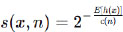
where E[h(x)] is the average path length, and c(n) is the average path length of unsuccessful searches in a Binary Search Tree;
4. Scores near 1 indicate anomalies; scores below 0.5 indicate normal instances.
Advantages: Linear time complexity, low memory requirements, effective in high dimensions, no distance or density calculations needed.
Limitations: Less effective for localized anomalies in datasets with complex regional densities; performance depends on appropriate sub-sampling size.
3.2.6.2. Feature Bagging for Outlier Detection
Feature bagging applies ensemble principles to outlier detection by constructing multiple base detectors on random subspaces of features, then aggregating their outputs [41].
How it works:
1. Randomly select subsets of features (typically √p or log2(p) features)
2. Train a base outlier detector (e.g., LOF or kNN) on each subspace
3. Aggregate outlier scores across ensemble members using averaging or maximum
Advantages: Handles high-dimensional data effectively, mitigates the curse of dimensionality, improves robustness, and naturally provides confidence intervals.
Limitations: Increased computational cost requires careful base detector selection.
3.2.6.3. Autoencoder-based Anomaly Detection
Autoencoders are neural networks trained to reconstruct input data through a low-dimensional bottleneck layer. The model learns to compress and reconstruct normal patterns. Anomalies exhibit high reconstruction error because they do not conform to learned normal representations (17).
How it works:
1. Train an autoencoder (encoder + decoder) on normal data only
2. For each test point, compute reconstruction error:

3. Points with reconstruction error exceeding a threshold (e.g., 95th percentile of training errors) are flagged as anomalies.
Advantages: Captures nonlinear relationships, adaptable to complex data, unsupervised, scales to large datasets.
Limitations: Requires large training samples, computationally intensive, “black box” with limited interpretability, sensitive to hyperparameter tuning.
Table 1 summarizes the comparative features of these advanced methods.
| Feature | Isolation Forest | Feature Bagging | Autoencoder |
|---|---|---|---|
| Time complexity | O(t × n × ψ) | O(m × n × d_sub) | O(epochs × n × p × h) |
| Memory usage | Low | Moderate | High (GPU recommended) |
| Handles high dimensions | √ Excellent | √ Good | √ Good (with regularization) |
| Interpretability | Moderate | Low | Very low (black box) |
| Requires training | Minimal | Moderate | Extensive |
| Best for | Large, high-D data | Very high-D, noisy data | Complex, nonlinear data |
| Output | Anomaly score (0-1) | Aggregated score | Reconstruction error |
3.3. Case Study: Outlier Detection in Simulated Medical Data with R
To bridge theory and practice, we present a fully reproducible medical case study using R. The simulated scenario involves detecting unusual patient laboratory profiles in a diabetes research dataset.
3.3.1. Study Scenario
Clinical question: Among patients being evaluated for diabetes risk, which individuals exhibit unusual laboratory profiles that may represent data errors, rare metabolic conditions, or exceptional clinical presentations?
Dataset simulation: We generate data for 1,000 patients with features including age, BMI, fasting glucose, HbA1c, triglycerides, and HDL cholesterol. We intentionally inject 3% anomalies representing:
- Type A (data errors): Extreme, physiologically impossible values
- Type B (rare conditions): Unusual combinations (e.g., low BMI with very high glucose)
- Type C (instrument errors): Systematic shifts in specific variables
The R code was presented in Appendix 1.
Figure 4 illustrates the simulated medical dataset after anomaly injection, where scatter plots and box plots demonstrate the separation between normal observations and artificially introduced anomalies. These visualizations provide an initial assessment of the distribution of anomalies before applying computational detection algorithms.
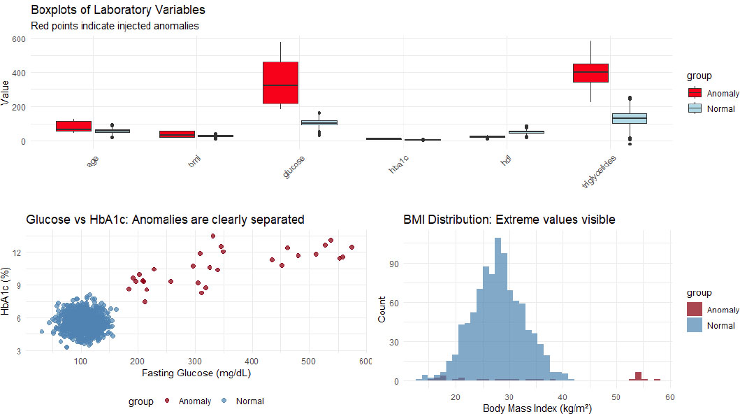
Scatter plot and boxplots of each variable with anomalies in red.
As shown in Figure 5, the kNN distance histogram reveals the distribution of neighborhood distances, and observations exceeding the selected threshold can be considered potential outliers.
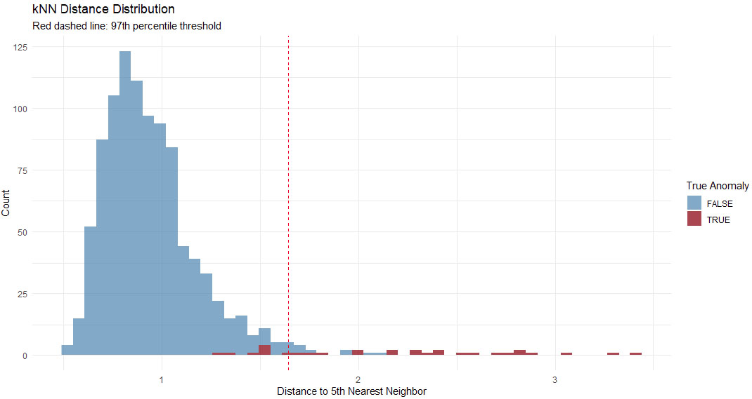
kNN distance histogram with threshold line.
Figure 6 presents the distribution of LOF scores, showing that density-based analysis assigns higher anomaly scores to observations in sparse regions.
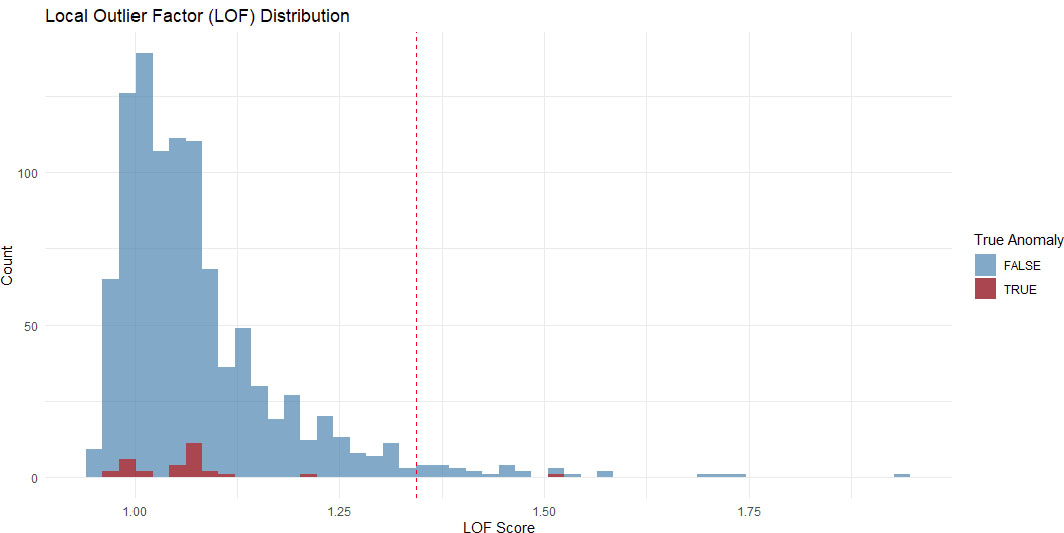
LOF score histogram showing outlier scores.
Figure 7 depicts the Isolation Forest anomaly score distribution, highlighting the ability of the algorithm to isolate rare observations through random partitioning.
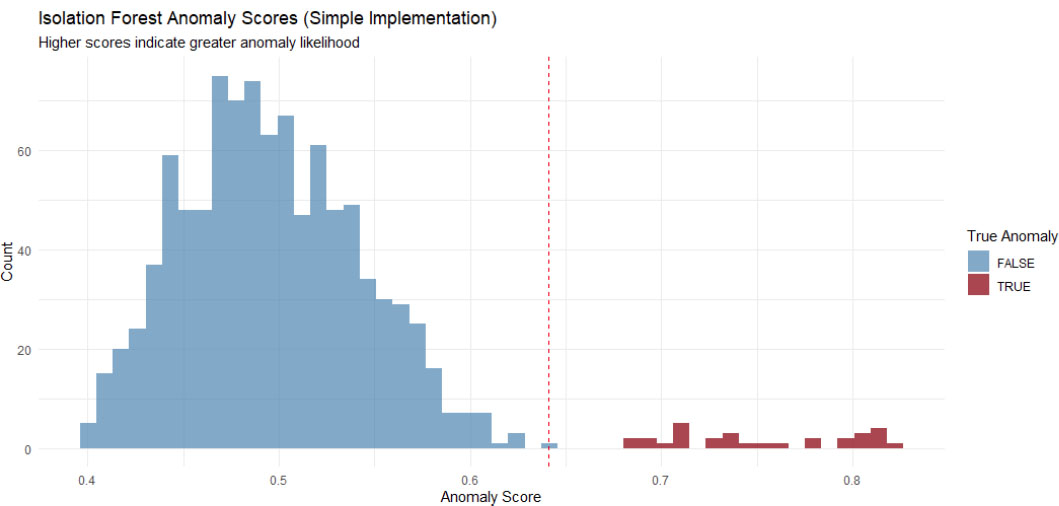
Isolation Forest score histogram.
Figure 8 shows the reconstruction error distribution obtained from the autoencoder-based approach, where samples with substantially higher reconstruction errors are identified as potential anomalies.
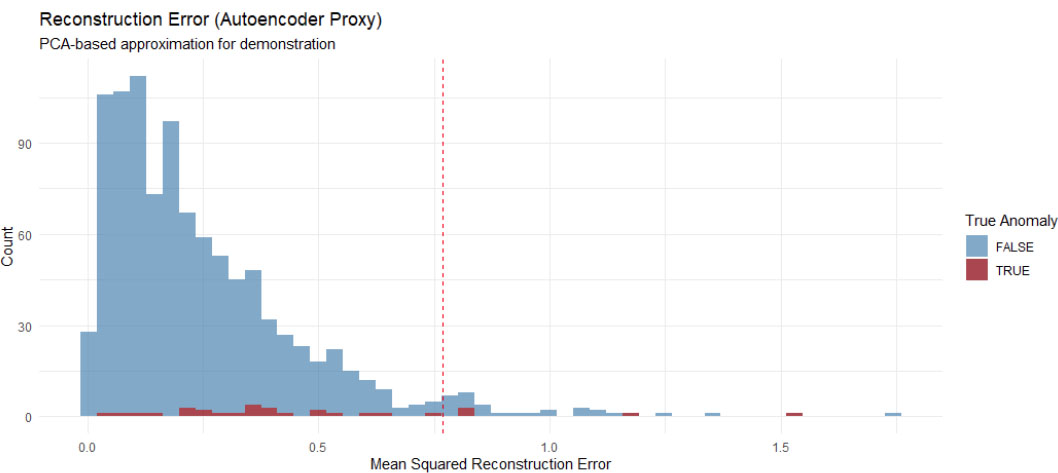
Reconstruction error plot (autoencoder proxy).
Figure 9 compares the ROC curves of the evaluated outlier detection approaches, providing an overall assessment of their discriminative performance in identifying injected anomalies.
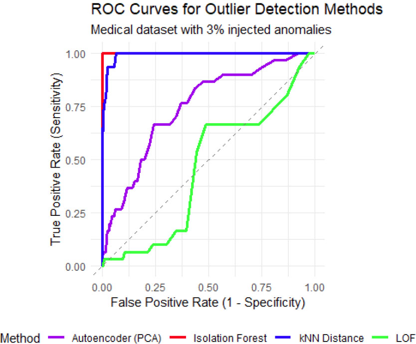
ROC curves comparing all four methods.
The simulation compared outlier detection methods on a synthetic medical dataset containing 3% injected anomalies. As shown in the boxplots, scatter plots, and histograms, the injected anomalies were visually distinct from normal observations. The ROC curves demonstrate that Isolation Forest substantially outperforms all other evaluated methods on this simulated medical dataset. The Isolation Forest ROC curve rises steeply, achieving a true positive rate exceeding 0.90 while maintaining a false positive rate below 0.05. LOF exhibits the second-best performance, followed by kNN Distance. The autoencoder (PCA proxy) shows the lowest discriminative ability, reflecting the limitations of linear reconstruction for capturing anomaly patterns. All methods perform significantly better than random classification (diagonal line, AUC = 0.5). These findings support Isolation Forest as the preferred method for multivariate outlier detection in clinical datasets, particularly when minimizing false positives is a priority.
4. SUMMARY AND COMPARATIVE ANALYSIS
There is considerable variation in the outlier detection environment, with distinct analytical perspectives for anomaly identification offered by each methodological family. Visual methods are dimensionally limited yet provide crucial, intuitive first attempts. Although they rely on strong distributional assumptions, statistical approaches offer mathematical rigor. Although distance-based methods are straightforward and non-parametric, they have trouble handling data with varying densities. Although density-based methods are highly effective in heterogeneous data contexts, they are computationally expensive. Although clustering-based approaches are effective and user-friendly, they do not optimize for outlier detection.
The following table provides a consolidated methodological category comparison (Table 2).
| Method Category | Key Principle | Assumptions | Pros | Cons | Best Suited For |
|---|---|---|---|---|---|
| Visual | Graphical identification of deviations | None | Intuitive, fast, no software required | Limited to low dimensions (1-3 variables), subjective | Initial data exploration |
| Statistical | Deviation from fitted model | Data follows known distribution (parametric) | Mathematical rigor, well-understood properties | Sensitive to model assumptions, suffers from curse of dimensionality | Low-dimensional data with known distribution |
| Distance-based | Points far from neighbors | None (non-parametric) | Simple, intuitive, no distribution assumed | Sensitive to parameters, struggles with mixed densities | Low-to-medium dimensional data with uniform density |
| Density-based | Points in low-density regions relative to neighbors | Local density reliably estimable | Handles clusters of different shapes/densities | Computationally expensive, parameter selection critical | Complex datasets with heterogeneous clusters |
| Clustering-based | Points not belonging to any cluster | Clusters represent “normal” data | Efficient, works as clustering by-product | Effectiveness depends on clustering quality | Large datasets where clustering is also of interest |
| Isolation Forest | Anomalies are few and different | Anomalies are sparse and distinct | Linear time, low memory, handles high dimensions | Less effective for localized anomalies | Large, high-dimensional datasets |
| Autoencoder | High reconstruction error | Normal data lies on a low-dimensional manifold | Captures nonlinear patterns, scalable | Black box, requires large samples, computationally intensive | Complex, nonlinear data (images, sequences) |
5. PRACTICAL RECOMMENDATIONS FOR MEDICAL RESEARCHERS
Detailed practical recommendations for medical researchers are provided in Table 3.
| Scenario | Recommended Method | Rationale |
|---|---|---|
| Small dataset (n < 100), few variables | Boxplots + Z-score | Simple, interpretable, clinically transparent |
| Medium dataset (100-1000), moderate dimensions | kNN + LOF | Balances performance and interpretability |
| Large dataset (>1000), many variables (>20) | Isolation Forest | Scalable, robust to high dimensions, minimal tuning |
| Complex nonlinear patterns, imaging data | Autoencoder | Captures intricate relationships, powerful |
| Real-time streaming data | Isolation Forest (incremental) | Fast, low memory, online adaptation possible |
Despite advances, several challenges remain:
1. High-dimensional data: Many methods suffer from the curse of dimensionality. Hybrid approaches combining feature selection with ensemble detection show promise.
2. Interpretability: Deep learning methods lack transparency. Explainable AI (XAI) techniques for anomaly detection represent an active research frontier.
3. Streaming data: Most methods assume static datasets. Online algorithms capable of adapting to concept drift are needed.
4. Labeled validation data: Rarely available in practice. Semi-supervised and self-supervised approaches are promising.
CONCLUSION
In the fields of data analysis and machine learning, outlier detection remains vital. From simple box plots and scatter plots to complex density-based algorithms such as LOF and MDEF, this review has traced the methodological progression. Different analytical perspectives are contributed by each methodology: statistical methods create model-based foundations, distance-based approaches offer geometric frameworks that are easy to understand, density-based techniques capture intricate local structures, and clustering-based methodologies combine pattern discovery and outlier detection. There is not a single best approach; instead, rigorous trade-off analysis is needed for selection. In addition to problem-specific interpretability and computational efficiency requirements, practitioners must consider data properties such as dimensionality, distribution, and volume. For example, whereas insurance claim fraud detection system developers would probably use sophisticated density-based or clustering approaches, medical researchers screening small laboratory datasets would start analyses with Z-scores and box plots. The key paradigm for successfully detecting rare, unique, and notable examples within complex data settings is ultimately provided by deliberate, iterative procedures that combine domain experience with rigorous methodological understanding.
FUTURE RESEARCH DIRECTIONS
Building on the reviewer's suggestions, priority areas for future research include:
1. Deep learning integration: Development of lightweight autoencoders and Variational Autoencoders (VAEs) for medical anomaly detection with improved interpretability.
2. Ensemble frameworks: Hybrid methods combining Isolation Forest with LOF for complementary strengths across different anomaly types.
3. Interpretable AI: SHAP and LIME adaptations for outlier detection models to explain why specific observations are flagged.
4. Benchmark datasets: Standardized medical anomaly detection benchmarks with realistic contamination rates and clinical ground truth.
5. Real-time clinical systems: Edge-deployable algorithms for continuous patient monitoring in ICU and wearable device settings.
6. Federated learning: Privacy-preserving outlier detection across multiple institutions without sharing raw patient data.
AUTHORS’ CONTRIBUTIONS
The authors confirms their contributions to the paper as follows: F.M.: Contributed to conceptualization, review, project management, writing the original draft, reviewing, and editing; S.B.: Contributed to writing the original draft, reviewing, and editing.
LIST OF ABBREVIATIONS
| KDE | = Kernel Density Estimation |
| LOF | = Local Outlier Factor |
| COF | = Connectivity-based Outlier Factor |
| ILFLO | = Influenced Outliernes |
| MDEF | = Multi-granularity Deviation Factor |
| RNN | = Reverse Nearest Neighbors |
| DBSCAN | = Density-based Clustering Methods |
ACKNOWLEDGEMENTS
Declared none.