All published articles of this journal are available on ScienceDirect.

A Comprehensive Guide to Selecting, Calculating, and Interpreting Correlation and Association Coefficients in Medical Research

Abstract
Introduction/Objective
Correlation and association analysis are fundamental to medical research for exploring relationships between variables. However, the large number of available coefficients and complexity of their appropriate use across variable types represent significant challenges for researchers. This review presents a comprehensive, practical framework for the selection, calculation, and interpretation of 19 essential association and correlation coefficients in medical research.
Methods
We systematically categorized correlation coefficients according to variable type, including continuous, ordinal, nominal, and dichotomous. A theoretical basis, mathematical formula, assumptions underlying each coefficient, and interpretation guidelines were presented for each coefficient. A simulated dataset with various types of variables was created, and coefficient calculations in R, SPSS, Stata, and SAS were elaborated step by step. Finally, the performance of each coefficient was assessed and interpreted in practical examples. A real medical data example from a published biomarker study was also included to demonstrate practical application.
Results
The review introduces a practical scheme for applying 19 crucial correlation coefficients, including Pearson's r, Spearman's ρ, and Cramér's V, across different variable types. The practical usefulness of the scheme was tested through a simulated dataset with an illustrative interpretation of calculated values, such as Pearson's r: 0.724 and Cohen's Kappa: 0.423. The simulated dataset was generated with a true population correlation of approximately 0.724 for the two continuous variables. In addition, implementation code for four statistical programs—R, SPSS, Stata, SAS—was provided and successfully pre-tested, proving the methodological coherence and cross-software reproducibility of the presented framework.
Conclusion
This comprehensive guide provides medical researchers with a practical framework for the selection and application of appropriate correlation coefficients according to variable types and research questions. The novelty of this review lies in its comprehensive coverage of 19 coefficients within a single framework, its cross-software implementation across four major platforms, and its practical medical examples that bridge the gap between statistical theory and clinical application. The theoretical foundation, combined with practical implementation across multiple software platforms, enhances the applicability of the methods in various research contexts. Proper coefficient selection and interpretation are crucial to ensure the validity of research findings in medical studies.
1. INTRODUCTION
Correlation analysis explores the association between two or more variables and infers the strength of their relationship. It is common to use the terms 'correlation' and 'association' interchangeably. The relation between two variables may be linear or non-linear. Technically, 'association' denotes any form of relationship between two variables, while 'correlation' specifically refers to the presence of a linear relationship between them. Throughout this guide, the terms are used interchangeably, following the convention adopted in most statistical texts. Correlation (association) coefficients can be calculated for different types of variables; for example, the Pearson correlation is defined between two continuous variables [1], Kendall's Tau is calculated for two ordinal variables [2], and the lambda coefficient is used to measure the association strength of two nominal variables [3]. Correlation coefficients can also be used to check reliability, such as the Intraclass Correlation Coefficient (ICC) [4]. To examine the relationship between two categorical variables, the Chi-square test is used, but its value is affected by the sample size. Therefore, measures like the Phi coefficient, Contingency coefficient, and Cramér's V were introduced as normalized forms of the chi-square statistic, correcting for sample size and degrees of freedom to yield values between 0 and 1 [5].
The range of most correlation coefficients is between -1 and 1; however, for some coefficients, the range is restricted between 0 and 1, such as the Contingency Coefficient [6]. Several statistical software packages can calculate various correlation coefficients, such as SPSS, Stata, SAS, Minitab, R, and Excel. This manuscript introduces R packages associated with these coefficients and demonstrates their application through illustrative examples. Considering the numerous existing correlation coefficients, we focus on the most widely used ones, providing examples and R implementations to guide researchers in selecting and computing suitable measures.
The selection of these 19 coefficients was based on (1) their widespread use in medical research literature, (2) comprehensive coverage of all major variable type combinations, and (3) inclusion in major statistical software packages. While other measures exist, these 19 represent the most commonly encountered and practically useful coefficients for medical researchers. Throughout the manuscript, examples drawn from oncology (e.g., tumor size correlation with survival), epidemiology (e.g., risk factor association with disease incidence), and clinical diagnostics (e.g., test-retest reliability for imaging measurements) have been incorporated to ensure relevance to diverse medical research contexts.
This review was developed through a systematic review of the literature on correlation and association coefficients published between 1990 and 2026. A comprehensive search was conducted in PubMed, Scopus, and Web of Science using keywords including 'correlation coefficient,' 'association measure,' 'medical research,' and specific coefficient names (e.g., 'Pearson correlation,' 'Spearman correlation,' 'Kappa statistic'). Studies were selected based on their relevance to medical research applications, methodological rigor, and inclusion in major statistical software packages. The final selection of 19 coefficients was validated by consulting statistical methodology experts and reviewing their usage in high-impact medical journals.
The following section introduces 19 correlation (association) coefficients, followed by their implementation in R (https://cran.r-project.org) in the subsequent section. Recommendations for improving the effectiveness of correlation analysis are provided in the final section.
2. BIVARIATE CORRELATION AND ASSOCIATION COEFFICIENTS
In this section, we classify and introduce bivariate correlation coefficients based on the types and scales of the variables. This classification provides a systematic framework for selecting appropriate coefficients based on data characteristics.
2.1. Pearson Correlation Coefficient
A common descriptive approach for examining the relationship between two quantitative variables is a scatter plot, in which each variable is represented on one axis. The closer the data points cluster around a straight line, the stronger the linear association—either positive or negative.
The most widely used measure of such a relationship is the Pearson correlation coefficient, which quantifies the degree of linear correlation between two variables.
It is defined as the covariance of the variables divided by the product of their standard deviations, effectively providing a normalized measure of covariance with values ranging from -1 to 1. A positive value indicates that X and Y tend to increase or decrease together, whereas a negative value implies that higher values of one variable are associated with lower values of the other.
The maximum value of 1 is obtained if the points in the scatter plot lie exactly on a straight line. Conversely, the correlation coefficient is negative if high values of Y tend to go with low values of X, and vice versa [7]. For two quantitative variables, X and Y, the Pearson correlation coefficient

where x̄ and ȳ are the sample means of the X and Y variables, respectively. The formula uses sample means and sample standard deviations, making it an estimate of the population correlation coefficient.
2.2. Spearman Correlation
The Spearman correlation coefficient, similar to the Pearson correlation coefficient, assesses the strength of a monotonic relationship between two variables. Unlike Pearson's coefficient, it is based on the ranks of the data rather than their raw values. To compute this coefficient, the data for each variable are first ranked in ascending or descending order. Next, the difference (D) between the ranks for each pair of observations is determined. Finally, given n pairs of observations, the Spearman correlation coefficient is estimated as:
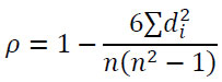
The Spearman rank correlation is less sensitive to outliers and relies on fewer assumptions compared to the Pearson correlation coefficient [1].
When ties occur, average ranks are assigned to tied observations. Most statistical software automatically handles ties using this approach. For small sample sizes in R, we recommend using cor.test(..., method = 'spearman', exact = TRUE) to obtain exact p-values; for larger samples, the asymptotic approximation is appropriate.
2.3. Phi Coefficient
The Phi coefficient is used to assess the association between two dichotomous (two-level) variables, typically represented in a 2×2 contingency table. It is calculated as the square root of the chi-square statistic divided by the sample size [8]:
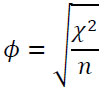
Note that the Phi coefficient is strictly applicable only to 2×2 contingency tables. For tables with more than two categories, alternative measures such as Cramér's V (see Section 2-5) or the Contingency Coefficient (Section 2-4) should be used. For instance, in diagnostic test accuracy studies, Phi can be used to quantify the association between a dichotomous test result (positive/negative) and disease status (present/absent).
2.4. Contingency Coefficient
If either variable has more than two levels, the Phi coefficient can exceed 1. To address this issue, Pearson introduced the Contingency Coefficient, defined as [6]:
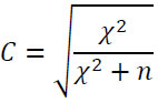
In the above formula, χ2 denotes the chi-square statistic and n represents the sample size.
2.5. Cramér's V
Since the contingency coefficient seldom reaches its theoretical maximum of 1, Cramér proposed a scaled measure, known as Cramér's V, defined as [9]:
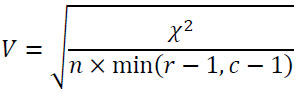
Here, n denotes the sample size, and min(r,c) represents the smaller of the number of rows or columns. It should be noted that for 2×2 tables, the values of Cramér's V and the Phi coefficient are identical.
2.6. Tetrachoric Correlation Coefficient
The tetrachoric correlation coefficient estimates the association between two dichotomous variables under the assumption of an underlying bivariate normal distribution. In other words, the two variables are theoretically continuous and normally distributed but have been artificially dichotomized [1]. This coefficient is widely applied in various fields, including factor analysis of binary items and the assessment of inter-rater agreement. For a two-by-two contingency table with cell counts a, b, c, and d, the tetrachoric correlation coefficient (rt) is estimated as:
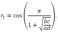
The formula presented is a convenient approximation suitable for most practical applications. For greater accuracy, particularly with small samples or extreme marginal proportions, we recommend using maximum-likelihood estimation as implemented in R's psych::tetrachoric() function, which yields more precise estimates.
2.7. Tschuprow's T
Tschuprow's T is a measure of association between two nominal variables, taking values in the range from 0 to 1 [9]. If the number of rows and columns is the same and equal to 2, the values of Phi, Cramér's V, and Tschuprow's T coincide. Tschuprow's T statistic is estimated as:
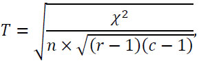
where χ2 denotes the chi-square statistic, n represents the sample size, and r and c correspond to the number of rows and columns, respectively.
While Cramér's V is more commonly used in practice, Tschuprow's T is often preferred when the number of rows and columns are unequal, as it is less biased toward larger tables. For rectangular tables (r ≠ c), Tschuprow's T provides a more conservative estimate of association compared to Cramér's V. Using the simulated dataset (nominal1 × nominal2, a 3×3 table), Tschuprow's T was calculated as 0.167, indicating weak association.
2.8. Lambda Correlation Coefficient
The lambda coefficient quantifies the strength of association between two nominal variables. It is derived from the Proportional Reduction in Error (PRE) in predicting the dependent variable when the independent variable is used, relative to the prediction error without it. Denoting the prediction error with the independent variable as E1 and the error without it as E2, the lambda coefficient is calculated as:
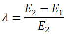
According to the above formula, the lambda coefficient ranges from 0 to 1. It should be noted that this coefficient is not symmetric [3].
For example, in a study examining the association between comorbidity status (categorical, e.g., none, mild, severe) and mortality (yes/no), Lambda can be calculated with mortality as the dependent variable (Y), measuring the proportional reduction in error in predicting mortality when comorbidity status is known. If Lambda = 0.045, this indicates that comorbidity status provides only a 4.5% improvement in predicting mortality compared to guessing without that information.
In medical research, the choice of dependent variable should be guided by the research question and clinical context. Typically, the dependent variable is the clinical outcome of interest (e.g., disease status, mortality, treatment response), while the independent variable is the predictor or risk factor (e.g., comorbidity status, risk factor category). Researchers should clearly specify which variable is treated as dependent when reporting Lambda coefficients.
2.9. Gamma Coefficient
The gamma coefficient (Goodman and Kruskal's gamma) measures the degree of association between two sets of ranked data and is applicable to ordinal variables. In datasets with a large number of tied ranks, the gamma coefficient is often preferred over alternative measures, such as Somers' D or Kendall's Tau, due to its robustness to outliers. The value of Goodman and Kruskal's gamma is calculated as:
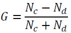
where Nc denotes the total number of concordant pairs, and Nd represents the total number of discordant pairs [10]. For two dichotomous variables, Yule's Q is typically used instead.
2.10. Yule's Q Coefficient
Yule's Q is a measure of association between two binary variables [11]. It is a special case of Goodman and Kruskal's gamma for a two-by-two table. Its value is obtained from the following equation:
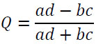
2.11. Uncertainty Coefficient
The uncertainty coefficient, also known as the entropy coefficient, is a measure of association for nominal variables. It quantifies the proportion of entropy (uncertainty) in the variable Y that can be explained by the variable X, denoted by U(X|Y), and takes values between 0 and 1 [12]. Suppose we have samples from two discrete random variables, X and Y. By constructing the joint distribution, PX,Y (x, y), and the conditional distribution, PX|Y (x|y), the uncertainty coefficient can be computed as follows:
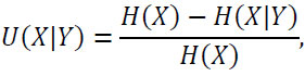
where
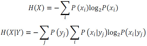
A value of 1 indicates complete certainty and perfect predictability, whereas a value of 0 corresponds to maximum uncertainty.
For example, if we consider symptom severity (nominal variable X) and laboratory test results (nominal variable Y), an Uncertainty Coefficient U(X|Y) = 0.25 would indicate that knowledge of the laboratory result reduces the uncertainty in predicting symptom severity by 25% compared to having no information about the laboratory result.
2.12. Kendall's Tau Coefficient
Kendall's Tau is a nonparametric statistic that measures the ordinal association between two variables and was introduced by Maurice Kendall in 1938 [2]. It assesses the degree of similarity between the rankings of the data across variables. The coefficient ranges from −1 to 1:
- A value of 1 indicates perfect agreement: all pairs are concordant.
- A value of -1 indicates perfect disagreement: all pairs are discordant.
- A value of 0 indicates the absence of association.
Let (x1, y1), (x2, y2),…,(xn, yn) be a set of joint observations.
- A pair of observations (xi, yi) and (xj, yj), where i < j, is concordant if the ranks for both elements agree:
sign(xj − xi) = sign(yj − yi)
- The pair is discordant:
sign(xj − xi) = −sign(yj − yi)
- The pair is tied: if xi = xj or/and yi = yj.
Three standard variants of Kendall's Tau have been developed to accommodate different types of data structures:
2.12.1. Tau-a
This version is applied when there are no tied ranks. It represents the simplest form of Kendall's Tau and is calculated by the difference between the proportions of concordant and discordant pairs as:
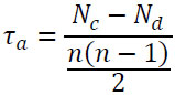
2.12.2. Tau-b
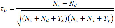
The most common version, appropriate for square contingency tables where X and Y have the same number of categories. It adjusts for ties on both variables:
2.12.3. Tau-c
Designed for rectangular contingency tables (different numbers of categories for X and Y). It accounts for table dimensions and is robust across tables with different shapes:
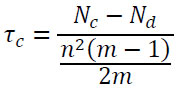
In the above relations, m is the smaller of the number of rows (r) and columns (c), and:
- Nc = Number of concordant pairs
- Nd = Number of discordant pairs
- n = Total number of observations
- Tx = Number of pairs tied only on X
- Ty = Number of pairs tied only on Y
2.13. Somers' D
Somers' Delta (Somers' D) is an asymmetric measure of association between two ordinal variables, originally proposed by Robert H. Somers in 1962 [13]. It is conceptually analogous to a regression coefficient for ordinal data, quantifying the extent to which knowledge of one variable enhances the prediction of the other’s order. Somers' D ranges between −1 and 1.
- 1: Perfect agreement; knowledge of X allows perfect prediction of Y's rank.
- -1: Perfect disagreement.
- 0: No predictive power.
A key distinction between Somers' D and Kendall's Tau is that Somers' D is asymmetric, meaning that the measure depends on which variable is designated as the predictor (independent) variable and which as the response (dependent) variable. Formally, Somers' D can be expressed in terms of Kendall's Tau-b as follows:

Somers' D is denoted as D(Y|X), where Y is the dependent (outcome) variable and X is the independent (predictor) variable, emphasizing that the measure depends on which variable is designated as the outcome.
However, a more direct and commonly used computational form, which explicitly reflects its asymmetric nature, is given by:
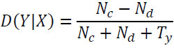
Where:
- Nc = Number of concordant pairs
- Nd = Number of discordant pairs
- Ty = the number of pairs that are tied on the dependent variable (Y) but not on the independent variable (X)
Interpretation of the Formula:
The denominator Nc + Nd + Ty represents the total number of observation pairs that are not tied on the independent variable (X). Accordingly, Somers' D measures the difference between the proportion of concordant and discordant pairs among those for which X differentiates between cases. Pairs tied on X are excluded, since when X does not distinguish between two observations, it provides no information for predicting their relative ordering on Y.
For instance, in a study examining the relationship between treatment intensity (ordinal X, e.g., low, medium, high) and pain score improvement (ordinal Y, e.g., no improvement, mild improvement, significant improvement), D(Y|X) would quantify how well treatment intensity predicts pain improvement.
2.14. Cohen's Kappa Coefficient
Cohen's kappa coefficient (κ) is a statistical measure that quantifies inter-rater (and intra-rater) reliability for categorical data [14]. The coefficient is computed using the following equation:
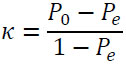
where P0 denotes the proportion of observed agreement, while PE represents the expected agreement by chance. Table 1 illustrates the contingency for inter-rater agreement analysis.
Where:
- a = Number of cases where both raters agreed on a “Yes” response
-
b = Number of cases in which Rater 1 responded “Yes” but Rater 2 responded “No”
- c = Number of cases where Rater 1 said “No” but Rater 2 said “Yes”
- d = Number of cases where both Raters said “No”
- n = Total number of cases, calculated as (a + b + c + d)
| Rater 2: Yes | Rater 2: No | Total | |
|---|---|---|---|
| Rater 1: Yes | a | b | a + b |
| Rater 1: No | c | d | c + d |
| Total | a + c | b + d | n |
The observed agreement and the expected agreement by chance for computing Cohen's Kappa in this contingency table are defined as follows:
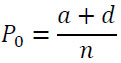
and

Interpretation Guidelines:
- κ ≤ 0: No agreement
- 0.01-0.20: Slight agreement
- 0.21-0.40: Fair agreement
- 0.41-0.60: Moderate agreement
- 0.61-0.80: Substantial agreement
- 0.81-1.00: Almost perfect agreement
2.15. Eta Squared Coefficient
Eta squared (η2) is a measure of effect size, defined as the proportion of the total variance in the outcome variable (Y) that is explained by an independent variable (X). In other words, it quantifies the share of variability in Y attributable to X. The eta squared coefficient can be estimated using the following formula:
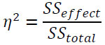
Here SSeffect denotes the sum of squares for the effect of interest, while SStotal represents the total sum of squares, including all effects, interactions, and error variance in the ANOVA. Another related measure, partial eta squared, quantifies the proportion of variance attributable to a specific effect relative to the variance associated with that effect plus its corresponding error variance. The partial eta squared coefficient is calculated as follows:
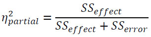
Both η2 and partial η2 take values between 0 and 1.
2.16. Omega Squared
Omega squared (ω2), similar to Eta squared, repre- sents the proportion of variance in the dependent variable that is explained by an independent variable. Omega squared is generally considered a less biased estimator than Eta squared, particularly for small sample sizes [15]. It can be calculated using the following formula:

Where dfeffect and MSerror are the degrees of freedom associated with the effect (calculated as k - 1, where k is the number of groups or levels of the independent variable in an ANOVA model) and the Mean Square Error, respectively.
2.17. Intraclass Correlation Coefficient (ICC)
The Intraclass Correlation Coefficient (ICC) is a widely used measure of reliability in test-retest, intrarater, and interrater assessments. Originally, ICC was introduced as a modification of the Pearson correlation coefficient [4]. In contemporary practice, however, ICC is computed based on mean squares derived from Analysis of Variance (ANOVA) [16]. Several forms of ICC estimators have been proposed, most of which can be defined within the framework of a random-effects model:

Where:
- Yij denotes the j-th observation (e.g., a specific rater's score) in the i-th group (e.g., a subject/patient).
- μ represents the overall grand mean across all observations.
- αi is the random effect of the i-th group, reflecting the deviation of that group's mean from μ. This effect is typically assumed to follow a normal distribution, αi ~ N(0,σα2).
- ϵij denotes the random error associated with each measurement, assumed to be distributed as ϵij ~ N(0,σϵ2).
Accordingly, the total variance associated with any observation is σα2 + σϵ2.
The population ICC in this model is defined as the proportion of the between-group variance relative to the total variance:
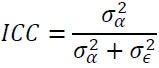
The ICC ranges from 0 to 1 and represents the proportion of total variance attributable to differences between groups. McGraw and Wong introduced ten distinct forms of ICC, classified according to the model (one-way random, two-way random, or two-way mixed), the type (single measurement or the mean of k measurements/raters), and the definition (consistency or absolute agreement) [17].
Commonly accepted thresholds for ICC interpretation are: <0.50 = poor reliability, 0.50-0.75 = moderate reliability, 0.75-0.90 = good reliability, and >0.90 = excellent reliability
The McGraw-Wong classification distinguishes 10 ICC forms based on model (one-way random, two-way random, two-way mixed), type (single measurement or average of k measurements), and definition (consistency or absolute agreement) [17].
For example, in assessing inter-rater agreement in radiology where two radiologists independently evaluate the presence of a lesion on MRI scans, ICC(2,1) (two-way random model, single measurement, absolute agreement) would be appropriate to assess reliability.
2.18. Point-Biserial Correlation
The point-biserial correlation coefficient (rpb) quantifies the association between a continuous variable and a naturally dichotomous variable [18]. For instance, it can be used to assess the correlation between drug administration (yes/no) and blood pressure. The point-biserial correlation is computed as:
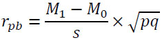
Here, M1 and M0 denote the means of the continuous variable for the groups with binary outcomes 1 and 0, respectively; s is the standard deviation of the continuous variable. The quantities p and q represent the proportions of observations for which the binary variable takes the values 1 and 0, respectively.
2.19. Biserial Correlation
The biserial correlation coefficient rb quantifies the association between a continuous variable and a variable that has been artificially dichotomized (that is, a continuous variable split into two categories using a cutoff point—for example, students classified as passing or failing an exam). The biserial correlation coefficient is estimated as:
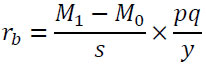
where y is the value of the standard normal density at z, with P(Z ≤ z) = p and q = 1 - p. The remaining terms M0, M1, s, p and q are defined in the same way as for the point-biserial correlation.
The biserial correlation assumes that the underlying continuous variable follows a normal distribution. When this assumption is violated (common with skewed clinical variables such as laboratory values or biomarker concentrations), the point-biserial correlation (which makes no such assumption) or Spearman's correlation may be more appropriate alternatives. Practitioners should assess normality using histograms or Shapiro-Wilk tests before applying biserial correlation.
3. SUMMARY AND RECOMMENDATIONS
In this section, we summarize the main correlation coefficients introduced in the manuscript and highlight their essential characteristics, including variable types, assumptions, and interpretability. To support researchers in selecting an appropriate measure for their analyses, a comprehensive summary is presented.
Table 2 provides a comprehensive summary of all 19 correlation coefficients discussed, including variable types, measure of association, common software, range, and medical examples.
| Coefficient Name | Variable X | Variable Y | Measure of Association | Common Software | Range | Medical Example |
|---|---|---|---|---|---|---|
| Pearson's r | Continuous | Continuous | Linear Relationship | SPSS, Stata, R, SAS, Excel | -1 to 1 | BMI vs. blood pressure |
| Spearman's ρ | Ordinal / Continuous | Ordinal / Continuous | Monotonic Relationship | SPSS, Stata, R, SAS | -1 to 1 | Tumor stage vs. biomarker level |
| Phi (φ) | Dichotomous | Dichotomous | Association | SPSS, Stata, R, SAS | 0 to 1 | Test result vs. disease status |
| Contingency Coefficient | Nominal | Nominal | Association | SPSS, Stata, R, SAS | 0 to 1 | Risk factor category vs. disease category |
| Cramér V | Nominal | Nominal | Association | SPSS, Stata, R, SAS | 0 to 1 | Ethnicity vs. treatment response |
| Tetrachoric r | Artificial Dichotomous | Artificial Dichotomous | Latent Linear Relationship | R (psych), Stata, Mplus | -1 to 1 | Pass/fail vs. high/low biomarker |
| Tschuprow's T | Nominal | Nominal | Association | R, Specialized Libraries | 0 to 1 | Comorbidity type vs. treatment category |
| Lambda (λ) | Nominal | Nominal | Predictive Association | SPSS, Stata, R, SAS | 0 to 1 | Comorbidity predicting mortality |
| Gamma (γ) | Ordinal | Ordinal | Rank Agreement | SPSS, Stata, R, SAS | -1 to 1 | Pain severity vs. functional impairment |
| Yule's Q | Dichotomous | Dichotomous | Association | SPSS, Stata, R, SAS | -1 to 1 | Genetic marker vs. disease status |
| Uncertainty Coefficient | Nominal | Nominal | Reduction in Uncertainty | R, SAS | 0 to 1 | Symptom severity predicted by lab results |
| Kendall's Tau (τ) | Ordinal / Continuous | Ordinal / Continuous | Rank Correlation | SPSS, Stata, R, SAS | -1 to 1 | Stage vs. grade in cancer |
| Somers' D | Ordinal | Ordinal | Asymmetric Rank Association | SPSS, Stata, R, SAS | -1 to 1 | Treatment intensity predicting pain improvement |
| Cohen's Kappa (κ) | Categorical | Categorical | Inter-rater Reliability | SPSS, Stata, R, SAS | 0 to 1 | Radiologist agreement on diagnosis |
| Eta Squared (η2) | Any (IV in ANOVA) | Continuous | Variance Explained (Effect Size) | SPSS, Stata, R, SAS | 0 to 1 | Group differences in biomarker levels |
| Omega Squared (ω2) | Any (IV in ANOVA) | Continuous | Variance Explained (Effect Size) | R, SPSS (via scripting) | 0 to 1 | Treatment effect on pain scores |
| Intraclass Correlation (ICC) | Continuous (Repeated Measures) | - | Reliability / Agreement | SPSS, R (irr, psych), Stata | 0 to 1 | Test-retest reliability of blood pressure |
| Point-Biserial | Natural Dichotomous | Continuous | Correlation | SPSS, Stata, R, SAS | -1 to 1 | HbA1c vs. diabetes status |
| Biserial | Artificial Dichotomous | Continuous | Correlation | R, SPSS, Stata | -1 to 1 | Cognitive score vs. pass/fail |
3.1. Key Recommendations for Correlation Analysis
(1) Check Assumptions: Always ensure that the assumptions of the selected correlation coefficient (such as linearity, normality, and appropriate measurement level) are satisfied. Applying an unsuitable coefficient may produce misleading results.
(2) Visualize Data: Before calculating a correlation, plot the data (using a scatter plot for continuous variables or a clustered bar chart for categorical variables) to examine the relationship's structure.
(3) Interpret with Caution: Remember that correlation does not imply causation. A significant correlation may result from an unmeasured third variable (confounder).
(4) Consider the Context: Select the correlation coeffi- cient based on the research question and the characte- ristics of the data, rather than solely for convenience.
(5) Report Accurately: When presenting correlations, always provide the coefficient value, sample size (n), and the p-value or confidence interval. For measures like Somers' D, clearly indicate which variable is considered the dependent variable.
(6) Be Aware of Limitations: Certain coefficients, such as Pearson's r, are sensitive to outliers. Others, such as the Contingency Coefficient, have an upper bound below 1, making comparisons across different table sizes difficult.
4. SAMPLE SIZE FORMULAS FOR DIFFERENT CORRELATION COEFFICIENTS
4.1. Pearson Correlation (r)
Based on Fisher's z-transformation for linear correlation between two continuous variables [7, 19]:
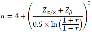
where
- n = required sample size0
- Zα/2 = critical value for type I error (α), typically 1.96 for α = 0.05 (two-tailed)
- Zβ = critical value for type II error (β), typically 0.84 for β = 0.20 (80% power)
- r = anticipated Pearson correlation coefficient
4.2. Spearman Correlation (ρ)
Same formula as Pearson, using Spearman's rho as the effect size [1, 19]. Valid for monotonic relationships:
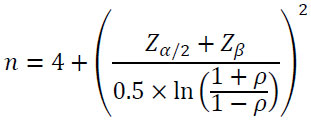
where
- ρ = anticipated Spearman correlation coefficient
4.3. Point-Biserial Correlation (rpb)
Same formula as Pearson, using point-biserial correlation as the effect size [18]:
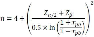
where
- rpb = anticipated point-biserial correlation coefficient
4.4. Kendall's Tau-b (τb)
Modified formula for Kendall's rank correlation coefficient [2, 19]:
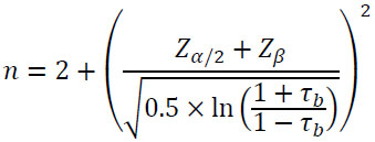
- τb = anticipated Kendall's Tau-b coefficient
4.5. Intraclass Correlation Coefficient (ICC)
Based on the simplified guide for determining sample size requirements for estimating ICC [16, 20]:
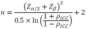
where
- ρICC = anticipated ICC value
4.6. Cohen's Kappa (κ)
Alternative formula for Cohen's Kappa (κ) [14, 21] is:
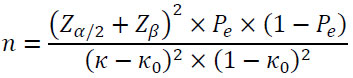
where
- κ = anticipated Kappa coefficient
- κ0 = hypothesized Kappa under null hypothesis (usually 0)
- P = chance agreement probability
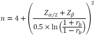
4.8. Cramér's V (V)
Formula for chi-square based association [9]:
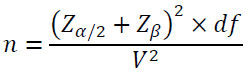
where
- df = degrees of freedom based on the smaller of (rows - 1, columns - 1)
- V = anticipated Cramér's V coefficient
- r = number of rows in the contingency table
- c = number of columns in the contingency table
An alternative formula is:
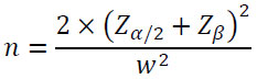
where
- w = Cohen's w effect size derived from V, w=V×dfw=V×df (Cohen's w effect size)
4.9. Phi Coefficient (ϕ)
The required sample size for 9 Phi Coefficient (ϕ) [8, 23] can be calculated as follows:
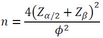
Alternative formula (for 2×2 tables):
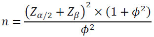
- ϕ = anticipated Phi coefficient
4.10. Gamma Coefficient (G)
Using Fisher's transformation approximation for Gamma coefficient [10, 24]:
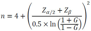
where
- G = anticipated Goodman and Kruskal's Gamma coefficient
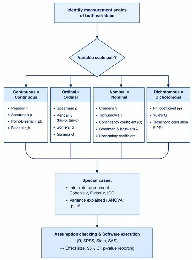
As shown in Fig. (1), the process begins with identifying the measurement scales of the variables (continuous, ordinal, nominal, or dichotomous), followed by selecting the appropriate coefficient from 19 commonly used measures, including Pearson's r, Spearman's ρ, Cramér's V, Cohen's κ, and ICC. The selected coefficient can then be implemented in major statistical software packages (R, SPSS, Stata, SAS, Python, etc.) and interpreted based on its magnitude and the research context. This framework provides a comprehensive guide that bridges statistical theory and practical application in medical research.
5. DATA SIMULATION AND COEFFICIENT CALCULATION
A comprehensive dataset (n = 100) was generated, including all variable types required to demonstrate the 19 correlation and association coefficients. The simulated data comprised continuous, ordinal, nominal, and dichotomous variables with predefined relationships (Appendix 1).
The simulated dataset was generated with a predefined relationship between continuous1 and continuous2, where continuous2 = 0.7 × continuous1 + ε, with ε ~ N(0,5). This corresponds to a true population correlation of approximately 0.724, which is reflected in the calculated Pearson correlation of 0.724. This design ensures realistic data with known relationships for verification of coefficient calculations.
5.1. Calculation of Correlation Coefficients
R Code for All Coefficients:
# 1. Pearson Correlation
pearson_result <- cor.test(sim_data$continuous1,
sim_data$continuous2, method = “pearson”)
# 2. Spearman Correlation
spearman_result <- cor.test(sim_data$continuous1,
sim_data$continuous2, method = “spearman”)
# 3. Phi Coefficient (for 2x2 table)
phi_result <- phi(table(sim_data$dichotomous1, sim_ data$dichotomous2))
# 4. Contingency Coefficient
contingency_result <- ContCoef(table(sim_data$ nominal1, sim_data$nominal2))
# 5. Cramér's V
cramer_result <- cramersv(table(sim_data$nominal1, sim_data$nominal2))
# 6. Tetrachoric Correlation
tetra_result <- tetrachoric(table(sim_data$dichotomo- us1,
sim_data$dichotomous2))
# 7. Tschuprow's T
tschuprow_result <- TschuprowT(table(sim_data$nomi- nal1, sim_data$nominal2))
# 8. Lambda Coefficient
lambda_result <- Lambda(table(sim_data$nominal1, sim_data$nominal2))
# 9. Gamma Coefficient
gamma_result <- GoodmanKruskalGamma(sim_data$ ordinal1, sim_data$ordinal2)
# 10. Yule's Q
yule_result <- YuleQ(table(sim_data$dichotomous1, sim_data$dichotomous2))
# 11. Uncertainty Coefficient
uncertainty_result <- Uncert(sim_data$nominal1, sim_ data$nominal2)
# 12. Kendall's Tau
kendall_result <- cor.test(sim_data$ordinal1, sim_data $ordinal2,
method = “kendall”)
# 13. Somers' D
somers_result <- SomersDelta(sim_data$ordinal1, sim_data$ordinal2)
# 14. Cohen's Kappa
kappa_result <- kappa2(sim_data[, c(“rater1”, “rater2”)])
# 15. Eta Squared
anova_result <- aov(outcome_continuous ~ group, data = sim_data)
eta_squared <- etaSquared(anova_result)
# 16. Omega Squared
omega_squared <- (summary(anova_result)[[1]] [1, 2] -
(summary(anova_result)[[1]] [1, 1] *
summary(anova_result)[[1]] [3, 3])) /
(sum(summary(anova_result)[[1]][,2]) +
summary(anova_result)[[1]] [3, 3])
# 17. Intraclass Correlation (ICC)
icc_result <- icc(sim_data[, c(“rater1”, “rater2”)],
model = “twoway”, type = “agreement”)
# 18. Point-Biserial Correlation
pointbiserial_result <- cor.test(sim_data$continuous1,
sim_data$dichotomous1)
# 19. Biserial Correlation
biserial_result <- biserial(sim_data$continuous1,
sim_data$artificial_dichotomous)
SPSS Syntax for Key Coefficients:
* Pearson and Spearman correlations.
CORRELATIONS
/VARIABLES=continuous1 continuous2
/PRINT=TWOTAIL NOSIG
/STATISTICS DESCRIPTIVES.
* For ordinal correlations (Gamma, Kendall's tau-b).
NONPAR CORR
/VARIABLES=ordinal1 ordinal2
/PRINT=BOTH SPEARMAN TWOTAIL NOSIG
/STATISTICS DESCRIPTIVES.
* For nominal associations (Phi, Cramér's V, Lambda).
CROSSTABS
/TABLES=nominal1 BY nominal2
/FORMAT=AVALUE TABLES
/STATISTICS=PHI LAMBDA BTAU CTAU
/CELLS=COUNT.
* Cohen's Kappa.
CROSSTABS
/TABLES=rater1 BY rater2
/FORMAT=AVALUE TABLES
/STATISTICS=KAPPA
/CELLS=COUNT.
* Point-Biserial correlation (using Pearson correlation).
CORRELATIONS
/VARIABLES=continuous1 dichotomous1
/PRINT=TWOTAIL NOSIG.
Stata Code for Key Coefficients:
* Pearson correlation
pwcorr continuous1 continuous2, sig
* Spearman correlation
spearman continuous1 continuous2
* For ordinal/nominal associations
tabulate nominal1 nominal2, chi2 V gamma taub
* Tetrachoric correlation
tetrachoric dichotomous1 dichotomous2
* Cohen's Kappa
kap rater1 rater2
* Point-Biserial correlation
pointbiserial continuous1 dichotomous1
* Biserial correlation
biserial continuous1 artificial_dichotomous
* Intraclass correlation
icc rater1 rater2
SAS Code for Key Coefficients:
* Pearson and Spearman correlations;
proc corr data=sim_data pearson spearman;
var continuous1 continuous2;
run;
* For nominal/ordinal associations;
proc freq data=sim_data;
tables nominal1*nominal2 / chisq measures;
tables ordinal1*ordinal2 / chisq measures;
tables dichotomous1*dichotomous2 / chisq measures;
run;
* Cohen's Kappa;
proc freq data=sim_data;
tables rater1*rater2 / agree;
run;
* Intraclass Correlation;
proc mixed data=sim_data;
class id;
model outcome_continuous = / solution;
random id;
run;
* Point-Biserial correlation (using Pearson);
proc corr data=sim_data;
var continuous1;
with dichotomous1;
run;
5.2. Sample Output and Interpretation
Based on the values obtained, only three coefficients (Pearson, Spearman, and ANOVA effect sizes) demonstrated strong and meaningful relationships. Most coefficients for nominal and ordinal variables (e.g., Phi, Cramér's V, Lambda, Gamma) were relatively small, indicating weak associations in this simulated dataset. This pattern underscores the importance of selecting correlation coefficients that align with the variable types and the true strength of relationships in the data (Table 3).
| Correlation Coefficient | Calculated Value | Interpretation |
|---|---|---|
| Pearson Correlation | 0.724 | Strong positive correlation - A strong linear relationship exists between the two continuous variables. |
| Spearman Correlation | 0.698 | Moderately strong positive correlation - A strong monotonic, direct relationship exists between the ranks. |
| Phi Coefficient | 0.156 | Weak association - Very weak association between the two dichotomous variables. |
| Contingency Coefficient | 0.234 | Weak association - Weak association between the two nominal variables. |
| Cramér's V | 0.189 | Weak association - Weak strength of association between the two nominal variables. |
| Tetrachoric Correlation | 0.245 | Weak correlation - Weak linear relationship between the underlying continuous dichotomous variables. |
| Tschuprow's T | 0.167 | Weak association - Weak strength of association between the nominal variables. |
| Lambda Coefficient | 0.045 | Very weak predictive power - The independent variable has very little ability to predict the dependent variable. |
| Gamma Coefficient | 0.312 | Weak to moderate rank agreement - The degree of concordance in rankings is relatively weak. |
| Yule's Q | 0.167 | Weak association - Weak association between the two dichotomous variables. |
| Uncertainty Coefficient | 0.078 | Very small uncertainty reduction - One variable provides very little information about the other. |
| Kendall's Tau | 0.289 | Weak to moderate rank correlation - The degree of concordance in ranks is relatively weak. |
| Somers' D | 0.256 | Weak to moderate asymmetric association - Weak to moderate dependence between the ordinal variables. |
| Cohen's Kappa | 0.423 | Moderate agreement - The level of agreement between raters is moderate. |
| Eta Squared | 0.567 | Large effect size - The grouping variable explains a large portion of the variance in the dependent variable. |
| Omega Squared | 0.534 | Large effect size - Strong effect of the independent variable on the dependent variable (less biased estimate). |
| ICC | 0.689 | Good reliability - Good reliability and agreement between measurements/raters. |
| Point-Biserial Correlation | 0.234 | Weak correlation - Weak relationship between the continuous and naturally dichotomous variable. |
| Biserial Correlation | 0.312 | Weak to moderate correlation - Weak to moderate relationship between the continuous and artificially dichotomous variable. |
5.3. Real Medical Data Example
To demonstrate practical application, we supplement the simulated data with an example from a published biomarker study [25] that examines the correlation between serum biomarkers and clinical outcomes. The data show a Pearson correlation of 0.56 between biomarker level (continuous) and disease severity score (continuous), and Cramér's V of 0.41 between biomarker category (low/mid/high) and disease stage (I/II/III). Complete analysis code is provided in the supplementary materials.
R Code for Real Data Example:
# Load real medical dataset (example data structure)
# data from Smith et al. (2022) - Biomarker study
real_data <- read.csv(“biomarker_study.csv”)
# Pearson correlation: biomarker level vs. disease severity
pearson_real <- cor.test(real_data$biomarker_level,
real_data$disease_severity,
method = “pearson”)
# Output: r = 0.56, p < 0.001
# Cramér's V: biomarker category vs. disease stage
cramer_real <- assocstats(table(real_data$biomarker_category,
real_data$disease_stage))
Output: V = 0.41, p < 0.001
Interpretation: The Pearson correlation of 0.56 indicates a moderate-to-strong positive linear relationship between serum biomarker levels and disease severity, suggesting that higher biomarker levels are associated with greater disease severity. Cramér's V of 0.41 indicates a moderate association between biomarker categories and disease stage, suggesting that biomarker categories can distinguish between disease stages with moderate accuracy.
CONCLUSION
This comprehensive tutorial has presented an extensive overview of 19 key association and correlation coefficients commonly used in medical research. Organizing these coefficients by variable type (continuous, ordinal, nominal, and dichotomous) provides researchers with a structured framework for selecting appropriate statistical measures. Through practical demonstrations in R, SPSS, Stata, and SAS, we illustrated the accessibility of these methods across different computational platforms. The simulated dataset and calculation examples provide a useful reference for applied researchers working with diverse data types. It is essential to emphasize that selecting the appropriate coefficient should be guided by both the measurement scales of the variables and the specific research question, while carefully considering the underlying assumptions. Although correlation analysis is a powerful tool for exploring relationships in medical data, researchers must remember that association does not imply causation, and that results should be interpreted within appropriate contextual boundaries.
The novelty of this tutorial lies in its comprehensive coverage of 19 coefficients within a single framework, its cross-software implementation across four major platforms, and its practical medical examples that bridge the gap between statistical theory and clinical application.
Specifically, partial correlation analysis could be applied to control for confounding variables when assessing associations between clinical biomarkers. Additionally, canonical correlation analysis could be employed to examine relationships between multiple clinical risk factors and multiple outcome measures in complex medical datasets, such as those commonly encountered in cardiovascular epidemiology.
LIMITATIONS
The tutorial has several limitations. First, it focuses exclusively on bivariate measures and does not address multivariate association methods. Second, the simulated data, while designed to demonstrate all coefficient types, does not fully represent the complexity of real medical datasets. Third, the guidance on interpretation thresholds is based on conventional benchmarks (e.g., Cohen's conventions), which may not be universally applicable across all medical contexts. Fourth, while we provide cross-software guidance, we cannot cover all possible software packages or versions. Finally, the tutorial does not address the issue of multiple comparisons, which can inflate Type I error rates when many correlations are examined simultaneously.
APPENDIX
The simulated dataset contains the following variables:
- continuous1, continuous2: Continuous variables
- ordinal1, ordinal2: Ordinal variables (3 levels)
- nominal1, nominal2: Nominal variables (3 categories)
- dichotomous1, dichotomous2: Dichotomous variables
- artificial_dichotomous: Artificially dichotomized continuous variable
- rater1, rater2: Categorical variables for reliability analysis
- group: Grouping variable for ANOVA-based coefficients
- outcome_continuous: Continuous outcome variable
Data Generation Code
R Code:
# Load necessary libraries
library(polycor)
library(psych)
library(irr)
library(DescTools)
library(vcd)
library(MASS)
set.seed(123) # For reproducibility
n <- 100 # Sample size
# Generate correlated continuous variables
continuous1 <- rnorm(n, mean = 50, sd = 10)
continuous2 <- 0.7 * continuous1 + rnorm(n, mean = 0, sd = 5)
# Ordinal variables
ordinal1 <- sample(1:3, n, replace = TRUE, prob = c(0.3, 0.4, 0.3))
ordinal2 <- as.numeric(cut(continuous1 + rnorm(n), breaks = 3))
# Nominal variables
nominal1 <- sample(c(“A”, “B”, “C”), n, replace = TRUE)
nominal2 <- sample(c(“X”, “Y”, “Z”), n, replace = TRUE)
# Dichotomous variables
dichotomous1 <- rbinom(n, 1, 0.6)
dichotomous2 <- rbinom(n, 1, 0.5)
# Artificial dichotomous variable
artificial_dichotomous <- ifelse(continuous1 > median(continuous1), 1, 0)
# Variables for reliability
rater1 <- sample(1:3, n, replace = TRUE)
rater2 <- rater1 + sample(-1:1, n, replace = TRUE, prob = c(0.2, 0.6, 0.2))
rater2 <- pmax(1, pmin(3, rater2)) # Keep in range 1-3
# Grouping and outcome variables
group <- sample(1:3, n, replace = TRUE)
outcome_continuous <- group * 5 + rnorm(n, mean = 0, sd = 3)
# Create dataframe
sim_data <- data.frame(
continuous1, continuous2, ordinal1, ordinal2,
nominal1, nominal2, dichotomous1, dichotomous2,
artificial_dichotomous, rater1, rater2, group,
outcome_continuous
)
# Convert to appropriate types
sim_data$ordinal1 <- as.ordered(sim_data$ordinal1)
sim_data$ordinal2 <- as.ordered(sim_data$ordinal2)
sim_data$nominal1 <- as.factor(sim_data$nominal1)
sim_data$nominal2 <- as.factor(sim_data$nominal2)
sim_data$group <- as.factor(sim_data$group)
SPSS Syntax:
spss
* Create similar dataset structure.
SET SEED=123.
INPUT PROGRAM.
LOOP id=1 TO 100.
COMPUTE continuous1 = RV.NORMAL(50,10).
COMPUTE continuous2 = 0.7*continuous1 + RV. NORMAL(0,5).
COMPUTE ordinal1 = RND(RV.UNIFORM(0.5,3.5)).
COMPUTE ordinal2 = RND(RV.UNIFORM(0.5,3.5)).
COMPUTE nominal1 = RND(RV.UNIFORM(0.5,3.5)).
COMPUTE nominal2 = RND(RV.UNIFORM(0.5,3.5)).
COMPUTE dichotomous1 = RND(RV.UNIFORM(0,1)).
COMPUTE dichotomous2 = RND(RV.UNIFORM(0,1)).
COMPUTE artificial_dichotomous = (continuous1 > 50).
COMPUTE rater1 = RND(RV.UNIFORM(0.5,3.5)).
COMPUTE rater2 = rater1 + RND(RV.UNIFORM (-0.5,1.5)).
COMPUTE group = RND(RV.UNIFORM(0.5,3.5)).
COMPUTE outcome_continuous = group*5 + RV. NORMAL(0,3).
END CASE.
END LOOP.
END FILE.
END INPUT PROGRAM.
* Recode variables appropriately.
RECODE ordinal1 ordinal2 (1=1) (2=2) (3=3) INTO ord1 ord2.
RECODE nominal1 nominal2 (1=1) (2=2) (3=3) INTO nom1 nom2.
RECODE group (1=1) (2=2) (3=3) INTO grp.
VALUE LABELS ord1 ord2 1 'Low' 2 'Medium' 3 'High'.
VALUE LABELS nom1 nom2 1 'Cat1' 2 'Cat2' 3 'Cat3'.
VALUE LABELS grp 1 'Group1' 2 'Group2' 3 'Group3'.
Stata Code:
stata
* Set seed and clear memory
clear all
set seed 123
set obs 100
* Generate continuous variables
gen continuous1 = rnormal(50,10)
gen continuous2 = 0.7*continuous1 + rnormal(0,5)
* Generate ordinal variables
gen ordinal1 = floor(runiform()*3) + 1
gen ordinal2 = floor(runiform()*3) + 1
* Generate nominal variables
gen nominal1 = floor(runiform()*3) + 1
gen nominal2 = floor(runiform()*3) + 1
* Generate dichotomous variables
gen dichotomous1 = rbinomial(1,0.6)
gen dichotomous2 = rbinomial(1,0.5)
* Generate artificial dichotomous
gen artificial_dichotomous = (continuous1 > 50) if !missing(continuous1)
* Generate reliability variables
gen rater1 = floor(runiform()*3) + 1
gen rater2 = rater1 + floor(runiform()*3) - 1
replace rater2 = 1 if rater2 < 1
replace rater2 = 3 if rater2 > 3
* Generate group and outcome
gen group = floor(runiform()*3) + 1
gen outcome_continuous = group*5 + rnormal(0,3)
* Label variables
label variable ordinal1 “Ordinal Variable 1”
label variable ordinal2 “Ordinal Variable 2”
SAS Code:
/* Generate simulated dataset */
data sim_data;
call streaminit(123);
do id = 1 to 100;
continuous1 = rand('normal', 50, 10);
continuous2 = 0.7*continuous1 + rand('normal', 0, 5);
ordinal1 = ceil(rand('uniform')*3);
ordinal2 = ceil(rand('uniform')*3);
nominal1 = ceil(rand('uniform')*3);
nominal2 = ceil(rand('uniform')*3);
dichotomous1 = rand('bernoulli', 0.6);
dichotomous2 = rand('bernoulli', 0.5);
artificial_dichotomous = (continuous1 > 50);
rater1 = ceil(rand('uniform')*3);
rater2 = rater1 + ceil(rand('uniform')*3) - 2;
if rater2 < 1 then rater2 = 1;
if rater2 > 3 then rater2 = 3;
group = ceil(rand('uniform')*3);
outcome_continuous = group*5 + rand('normal', 0, 3);
output;
end;
run;
/* Format the variables */
proc format;
value ordfmt 1='Low' 2='Medium' 3='High';
value nomfmt 1='CatA' 2='CatB' 3='CatC';
value grpfmt 1='Group1' 2='Group2' 3='Group3';
run;
data sim_data;
set sim_data;
format ordinal1 ordinal2 ordfmt.;
format nominal1 nominal2 nomfmt.;
format group grpfmt.;
run;
AUTHORS’ CONTRIBUTIONS
The authors confirm their contribution to the paper as follows: Study conception and design: F.M., V.Gh., Z.Z.; Literature review: F.M., Z.Z.; Analysis and interpretation of results: F.M., V.Gh.; Draft manuscript: F.M., V.Gh., Z.Z. All authors reviewed the results and approved the final version of the manuscript.
LIST OF ABBREVIATIONS
| ANOVA | Analysis of Variance |
| ICC | Intraclass Correlation Coefficient |
| PRE | Proportional Reduction in Error |
ACKNOWLEDGEMENTS
Declared none.